Multi-Scale Microfluidics for Transport in Shale Fabric


1
Energy Resource Engineering, Stanford University, Stanford, CA 94305, USA
2
Department of Geology, University of Illinois at Urbana-Champaign, Urbana, IL 61801, USA
*
Author to whom correspondence should be addressed.
Energies 2021, 14(1), 21; https://doi.org/10.3390/en14010021
Submission received: 28 October 2020
/
Revised: 10 December 2020
/
Accepted: 15 December 2020
/
Published: 23 December 2020
(This article belongs to the Special Issue Multiscale and Multiphysics Processes in Unconventional Formations 2020)
Abstract
:We develop a microfluidic experimental platform to study solute transport in multi-scale fracture networks with a disparity of spatial scales ranging between two and five orders of magnitude. Using the experimental scaling relationship observed in Marcellus shales between fracture aperture and frequency, the microfluidic design of the fracture network spans all length scales from the micron (1 ) to the dm (10 dm). This intentional ‘tyranny of scales’ in the design, a determining feature of shale fabric, introduces unique complexities during microchip fabrication, microfluidic flow-through experiments, imaging, data acquisition and interpretation. Here, we establish best practices to achieve a reliable experimental protocol, critical for reproducible studies involving multi-scale physical micromodels spanning from the Darcy- to the pore-scale (dm to m). With this protocol, two fracture networks are created: a macrofracture network with fracture apertures between 5 and 500 m and a microfracture network with fracture apertures between 1 and 500 m. The latter includes the addition of 1 m ‘microfractures’, at a bearing of 55°, to the backbone of the former. Comparative analysis of the breakthrough curves measured at corresponding locations along primary, secondary and tertiary fractures in both models allows one to assess the scale and the conditions at which microfractures may impact passive transport.
1. Introduction
Presently, in the United States and increasingly around the world, a significant volume of oil and natural gas is being produced from unconventional reservoirs that are commonly dominated by shale lithology [1]. Shales are ultrafine-grained sedimentary rocks that exhibit variability in structural and chemical features across a broad range of characteristic length scales [2,3,4]. They have multi-modal pore size distributions varying over multiple length scales (10 to 10 m [5,6,7,8,9,10,11]), where nano-scale pores are most common and can be interparticle, intraparticle or even inside the organic matter itself [12]. The rock fabric is very tight and compact with nanometer-scale pathways and nano-Darcy permeability [3,13], but it is inundated with innumerable natural fractures. This fracture network follows a characteristic power-law relationship between the fracture aperture and frequency [14,15], which dictates its transport properties [16]. Following this power-law relation, the prevalence of smaller ’micro-fractures’ are expected in these fabrics but they are extremely difficult to resolve through common characterization techniques.
Connected pathways are engineered in these low-permeability rocks by injecting high-pressure acidic fluid, often followed by a ‘shut in’ or accumulation period, and finally commercial recovery of hydrocarbons [17]. The high-pressure fluid physically breaks the rock, while the acidity chemically interacts with the fracture surfaces, resulting in the evolution of these flow channels and their apertures [18,19,20] over time. The result is a transient growth and connection of the natural fracture fabric, leading to complex fracture geometries [21,22,23] through which the hydrocarbons are transported to the wellbore and produced on the surface.
Theoretical models for hydraulic fracturing have been developed for the better part of the last century, yet current planar fracture models are incapable of capturing the behavior of hydraulic and natural fracture interactions [24]. Fully 3D models that can accurately predict what happens when flow paths are suddenly forced through natural fracture fabrics have not been successfully developed yet [17]. Impediments to further progress currently include the difficulties associated with encapsulating the range of length scales that describe shale heterogeneity and branching and intersection of fractures. Furthermore, the process of simulating fluid transport in shale is computationally exhaustive due to the dependence of macroscopic transport properties on the underlying micro- and nano-structures. Thus far, volume-averaging and other upscaling methods are lacking for this feedback leading to a necessity to resolve several orders of magnitude in length scales [25,26]. As described above, these micro- and nano-structures are extremely difficult to resolve, but the power-law relationship between the fracture aperture and frequency indicates that they are highly prevalent in these rock fabrics.
An immediate challenge is then to quantitatively predict the behavior of solutes transported through these multi-scale fracture networks, including hydrocarbons and the ions generated by acidification of the reservoir. The geometry of the fracture network is reflected in advective mass transfer fluxes which span several orders of magnitude [27,28], network-scale mixing at the fracture intersections [29] and dispersion as a result of the velocity profile between the bounding walls in a fracture and along the rough fracture surface [30,31]. For shale rocks, this is further complicated by the presence of reactive minerals on the fracture surface [32], nanometer-scale pore sizes, an ultra-low permeability rock matrix and a plethora of natural and artificial fractures of varying aperture size and length [33,34]. Experimentally, imposing appropriate boundary conditions (be it ambient pressure at the outlets or varying concentration at the inlet) still remains an open challenge due to the multi-scale fabric of the system.
Direct observations of the propagation of solutes through fracture networks, which honor the natural fabric of shales, are necessary to further progress towards quantitative modeling of these complex structures and the reactive transport processes that occur within them. Physical micromodels have often been used to study the interplay among physics, chemistry and topology in different dynamical flow regimes and their impact on solute transport [35,36,37]; however, the inherent multi-scale nature of the fracture network makes the experimental design difficult. Most of the existing micromodel fabrication techniques, which are based on either material removal (e.g., etching [35,38]) or material addition (e.g., lithography [39]), create a quasi-two-dimensional structure where the aspect ratio between the spacing and the depth of the feature is dictated by the fabrication technique and accuracy. A slender feature (depth ≫ width) or a wide feature (depth ≪ width) is associated with its own challenges and the fabrication method of choice. When fracture aperture in a network spans over multiple orders of magnitude, finding an optimal fabrication protocol is particularly challenging. Implementation of fluid injection and boundary conditions brings additional complexity into these multi-scale micromodel experiments. Notable issues arise due to the orders of magnitude difference between the micromodel’s interior space (volume) and the exterior pumping and tubing system. Furthermore, significant uncertainty [36,40] is introduced through microscopes which are used for imaging and visualization of the micromodels; the image quality is a function of the spatiotemporal resolution and lighting. The multi-scale nature of these natural fracture networks require measurements to be taken at multiple locations for which the stage must be moved, compounding this uncertainty. Thus, the establishment of a reliable experimental protocol is crucial for reproducible studies involving multi-scale physical micromodels.
The objective of the present paper is to demonstrate that a physical micromodel can be constructed such that the power-law relationship describing shale fracture size and distribution is preserved over multiple orders of magnitude in length, and that the solute tracers can be reliably and reproducibly tracked through this system in real time at resolutions sufficient to extract breakthrough curves (BTCs) and relevant parameter values. This study offers a proof of concept which is vital to direct observation of flow and transport in a class of physical structures that are naturally occurring, economically significant and computationally challenging. For this, we employ soft photolithography to fabricate micromodels that consist of fracture apertures spanning two to three orders of magnitude with the dimensional scale spanning five orders of magnitude: smallest fracture with 1 m aperture, largest fracture with 500 m aperture and the fracture network length of ∼100 mm. The experimental platform consists of maintaining a steady-state injection of fluorescent dye, which is then visualized and recorded by an inverted microscope using a CMOS camera.
In this paper, we explore the capacity to generate reproducible steady-state flow fields in shale fracture networks, demonstrate successful recovery of solute breakthrough and highlight the difficulties associated with micromodel fabrication and experimental flooding design. Section 2 describes the design and fabrication of the micromodels, the experimental setup and solute concentration field visualization. Section 3 presents the experimental results including uncertainty quantification. Section 4 analyzes the challenges and functionality of this experimental design and offers a set of benchmark metrics to validate appropriate behavior in this class of physical models across different scales and within different transport regimes.
2. Materials and Methods
2.1. Micromodel Design and Fabrication
Gale et al. [14] empirically observed that in natural rock fracture fabrics the number of fractures decreases as the size of the fractures increases. Specifically, the relationship between the fracture aperture b (in mm) and its corresponding frequency f (frac/m) obeys a power law of the general form
where is the scaling coefficient and is the scaling exponent.
Figure 1 shows both the experimentally observed scaling relationship found in Marcellus shales (square markers) [14] and the corresponding fitted exponential function (dashed red line) described by
The microchip design is based on extrapolating this scaling relationship to smaller sizes (Figure 1, circles), while anchoring the largest fracture aperture at the cm scale, to obtain a micromodel with a hierarchy of fractures spanning between 2 and 3 orders of magnitude in aperture. The dimensional scale of the network itself spans 5 orders of magnitude with a fracture length of ≈ 100 mm and the smallest feature of 1 m. To the best of our knowledge, this is the first microfluidic system to operate at a macro or Darcy scale, while individual fracture apertures can be as small as 1 m.
Two fracture networks are created for this study (Figure 2): (i) a macrofracture network (here referred to as MFN) with fracture apertures between 5 and 500 m; and (ii) a microfracture network (FN) with fracture apertures between 1 and 500 m. The FN includes the addition of 1 m ‘microfractures’, at a bearing of 55°, to the MFN’s backbone. The geometry of the network and contact angles between intersections is based on an actual fractured shale sample (Figure 7 of [14] and Figure 10 of [41]). Figure 2 shows the structure of the two micromodels and Table 1 lists the number of fractures of a given aperture for the MFN and the FN micromodels. The actual patterns are shown in Figure 2. All the circular markers on the rim of the fracture networks are the micromodel inlet and outlet ports indicated in red and blue, respectively.
The PDMS (polydimethylsiloxane) micromodels were fabricated at the Stanford Nanofabrication Facility through photolithography. The PDMS fabrication process involves two major steps: (i) fabricating the silicon wafer mold with patterns etched on it; and (ii) molding the PDMS using the silicon wafer mold. The MFN and FN were printed separately onto two glass photo masks (Martin Photomask, Escondido, CA, USA), with the fabrication of both micromodels following the same procedure. First, we prepared a photo resist mixture by combining 60% (by volume) SU-8 2025 and 40% (by volume) SU-8 2000.5 (MicroChem, Newton, MA, USA). A silicon wafer was then spin-coated with the photo resist mixture before being exposed to UV light with the printed mask covered on top of it. A post-exposure baking step solidified the fracture network pattern on the silicon wafer and then the silicon wafer was placed in SU-8 developer to dissolve the excessive photo-resist. Finally, it was hard baked on a hot plate (180 °C for 30 min), which resulted in a quasi-two-dimensional geometry with a height m. Such a height is determined by optimizing the ratio between the fracture aperture and vertical wall height ().
In a typical PDMS micromodel, a large ratio results in a collapsed channel (top wall touching the bottom wall) and a small ratio results in poor vertical resolution of the fracture feature (i.e., roughness of the vertical wall is significantly increased). To determine the optimal in these multi-scale models, we tested a variety of compositional ratios of the photo resist (the mixture of SU-8 2025 and SU-8 2000.5). When we used 100% SU-8 2025, the feature height was ∼25 m, which provided a finely resolved m fracture but poorly resolved m for the FN. By increasing the SU-8 2000.5 volume ratio to 10%, the was reduced to ∼20 m. When the composition reached 40 % SU-8 2000.5, we achieved an optimal height of m, where both the 1 m and m fractures were adequately resolved. Notably, through this analysis, we found that the resultant feature height changes non-linearly with the fabrication protocol. For instance, if we reduced the spin-coat speed by half, the final was reduced by more than half. Adjusting the mixture composition of the same type photo resist while keeping the same protocol allowed us to identify the optimal height.
Once the silicon wafer mold was prepared, we mixed 184-PDMS base and 184-PDMS curing agent (Dow Corning, Midland, MI, USA) with mass ratio 10:1 and poured it into the wafer mold. After curing at 70 °C for 3 h, the PDMS was patterned with the same concave geometry. Holes were punched in all the port locations shown in Figure 2 and the PDMS micromodel was plasma-bonded to a glass wafer. The bonding was performed by activating the PDMS and glass surface using air-plasma and baked (90 °C for 8 h) to secure the bonding. Once the micromodel was bonded, it was submerged in a filled crystallizing dish filled with DI water and placed in a desiccator connected to a vacuum pump. The air contained inside the micromodel formed bubbles that were less buoyant than the surrounding water phase, causing them to rise towards the surface. The micromodel was left in the desiccator for 1–2 days to ensure that no air bubbles were observable on the surface of the micromodel or in the DI-water contained in the crystallizing dish. The micromodel was then considered ready for fluid injection.
2.2. Flow-Through Experiment Design
All experiments were run in the Multi-scale Physics in Energy Systems (MPES) laboratory at Stanford University. After saturation, steady-state flow conditions were achieved through continuous fluid injection at the inlet port (red port in Figure 2) while free flow conditions at constant pressure were enforced at all the outlet ports (blue ports in Figure 2). The design allowed easy modification of the boundary conditions by switching the ports from inlets to outlets and vice versa, as desired. To impose a single phase constant pressure condition, all the outlets were connected to a waste bottle, which was kept at the same elevation as the micromodel and open to the atmosphere (shown in Figure 3A). We found that this was an essential aspect of the experimental design because the individual outlets each connect to fractures of different widths. If these outlets were simply left open, the air–water interface formed at each outlet would have unique radii and therefore the fluid within the micromodel locally would experience a unique pressure boundary at each outlet. Connecting all outlets to a common waste bottle mitigated these small but consequential non-uniformities in pressure at the outlets across the micromodel and thus facilitates stable flow.
The experimental design and tubing systems are shown in Figure 3A. One high precision syringe pump (PHD 2000, Havard Apparatus, Holliston, MA, USA) was used for injection and one multi-channel syringe pump (NE-1600, New Era Pump Systems Inc., Farmingdale, NY, USA) was used for cleaning. Two 1 mL glass syringes (Hamilton, MA, USA) were attached to the high precision HA pump and one 1 mL glass syringe was attached to the NE syringe pump. One syringe contained the fluorescent dye and the other two were filled with DI-water. The three syringes were connected to two four-way valves (Valve I and Valve II) that were controlled by two servo motors with an Arduino® control board. The servo motors were programmable and controlled to switch the valves on simultaneously, thus minimizing the flow perturbation in the micromodel between different injection patterns.
The micromodel was mounted on the microscope stage and the entire fracture network was visually inspected to ensure homogeneity of the saturating fluid. Three injection phases were performed (Figure 3B): cleaning, flow stabilization and solute injection. The cleaning phase was initiated after the completion of any previous experiment and was used to remove any solute remaining in the micromodel and tubing system. Valve I was switched to the main channel while Valve II was switched to by-pass (Figure 3B). Once the micromodel was cleaned and saturated with DI water, the flow stabilization phase was initiated. DI water and fluorescent dye, each contained in separate syringes of equal volume mounted on the same syringe pump, were injected at the same flow rate. We found that injecting one pore volume of DI water ensured stable steady-state flow in the micromodel. For all of our micromodels, we injected a minimum of one pore volume (∼2–30 min depending on the flow rate) to ensure flow stability inside the micromodel before the dye was introduced. The dye was injected by switching both valves as follows: Valve I was switched to by-pass and Valve II was switched to the main channel, thus omitting any interruption in flow or any perturbation to the pressure gradient across the micromodel. Image acquisition was initiated at the same time.
2.3. Imaging and Data Acquisition
In each experimental run, the micromodel was placed on the inverted microscope (Ti-E, Nikon Instruments Inc., Melville, NY, USA), equipped with a motorized stage. Light was emitted by a light source unit (SOLA SE II, Lumencor Inc., Beaverton, OR, USA) and passed through a filter cube (C-FL GFP, Nikon Instruments Inc., Melville, NY, USA), which filtered out all the wavelengths except for green light. The light, incident on the micromodel, excited the Alexa-488 flourescence dye (ThermoFisher Scientific, Inc., San Diego, CA, USA) contained in the fracture network. The light emitted from the dye was magnified by an 10× objective (CFI60 Plan Apochromat Lambda, Nikon Instruments Inc., Melville, NY, USA) and captured by a CMOS camera (Hamamatsu Flash LT Monochrome, Hamamatsu, San Jose, CA, USA) operating at a 100 ms exposure time. The light intensity was used to map the concentration field in the micromodel, where a higher dye concentration emitted more light and resulted in a higher local light intensity. To minimize light scattering and ambient light influence, the entire micromodel was covered with a dark foil which absorbed most of the transmitted light.
The motorized stage was programmed to acquire images at nine locations sequentially, labeled as P1–P3, A1–A3 and A10–A12 (Figure 4A), located on the primary, secondary and tertiary fractures, respectively. These locations were chosen for the present study as they were relatively close to the inlet and thus BTCs were captured relatively quickly. Further, the points were chosen as pairs located along several fractures, e.g., P2 and P3 were one pair of upstream and downstream points located on the 500 m fracture. This paired comparison allowed us to systematically verify consistency in transport along the fracture network. The comparison between the MFN and FN results supported exploration of the effects of the smallest microfractures in the flow cell. The location coordinates and connected fracture widths are presented in Table 2.
For each location, we separately measured the average light intensity within each individual blue and orange box (Figure 4A) at the north (N), east (E), south (S) and west (W) branch. The average light intensity () was measured inside each blue box shown in Figure 4A (right). Measurements in the orange boxes provided the control as they accounted for the local variation in the background () on the PDMS wall without the influence of the fluid and/or dye solute. We found that significant variations in background can occur across the micromodel due to the distance between the measuring locations, the spatial and temporal non-uniformity of the light source [36] and the local imaging conditions [40]. As a result, the light intensity at each measurement point needed to be locally corrected. The corrected light intensity () (Figure 5-Top) was therefore calculated as:
A quadratic regression smoothing filter was applied to the raw data to eliminate minor fluctuations. The data were labeled in the following format:
where MFN/FN indicates the fracture network, XX is the corresponding flow rate in L/h, YY is the measurement location and Z is the branch (i.e., N, S, E, W) of the fracture where the intensity is recorded. To compare the BTCs, the intensity was converted to dimensionless concentration (C) according to the linear relationship
where and are unknown constants. The intensity at the two solute concentration extrema, i.e., 100% water saturation () and 100% dye saturation (), can be solved simultaneously to give the dimensionless concentration C,
where
The physical time () was converted to dimensionless time (t) following Ogata and Banks [42]:
where and are the average velocity and molecular diffusivity, whose values are given in Table 3, and is the arrival time, defined as the time instance when the concentration reaches .
In Figure 5, we show an example of the how raw data were processed to map light intensity measurements into breakthrough curves. Figure 5 shows the measurements at the east branch of A1 with flow rate L/h in the FN (FN, Q10-A1-E). In the top inset, we plot both the measured light intensity () and the background () intensity as functions of time; the middle inset shows the calibrated concentration as a function of physical time, and the bottom one shows the BTC as a function of the dimensionless time.
3. Results
3.1. Experiment Reproducibility and Measurement Error
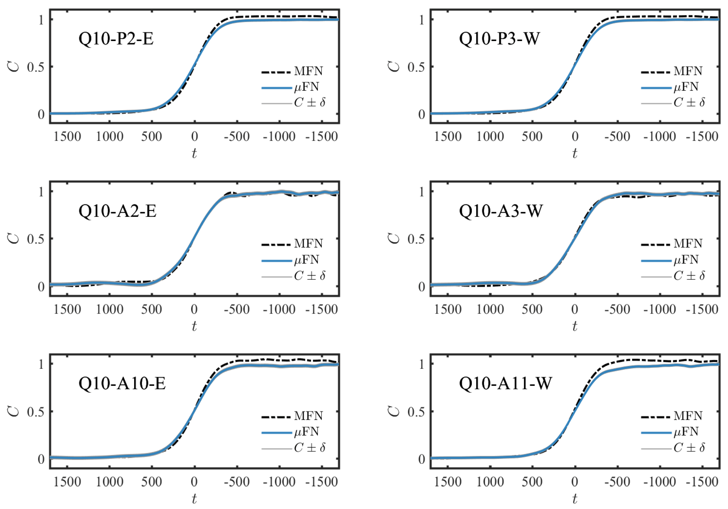
These micromodels are uniquely complex and include a version (FN) which spans five orders of magnitude in length scales. Thus, it is first necessary to assess the robustness and reproducibility of the experimental protocol. We quantify measurement error in the BTCs by conducting five replicate measurements under the same flow conditions in each of the four branches (N, S, E and W) of the intersection at the nine locations in FN (P1,P2, P3, A1, A2, A3, A10, A11 and A12). This was carried out by replicating the FN at flow rate Q = 10 L/h (FN, Q10) four additional times (FN, Q10 R1–R4). Table 4 summarizes the flow rate, Peclét number and arrival time for all the experiments including the repeated runs in FN, Q10 (R1, R2, R3 and R4). As shown in Table 4, repeated experiments within the same micromodel and under the same experimental condition still show uncertainty in arrival time (the P1 point arrival time of the FN varies 300–430 min). At a flow rate of Q = 10 L/h, this difference (∼130 min) in the arrival time corresponds to ∼20 pore volume of the micromodel; however, such volume only corresponds to ∼7 mm length inside the exterior tubing. Thus, differences in the absolute arrival time between experiments can be caused by the difference in the initial location of the dye plume. This variation in the repeated experiments also indicates that an error analysis is a necessity for such a multi-scale micromodel experiment.
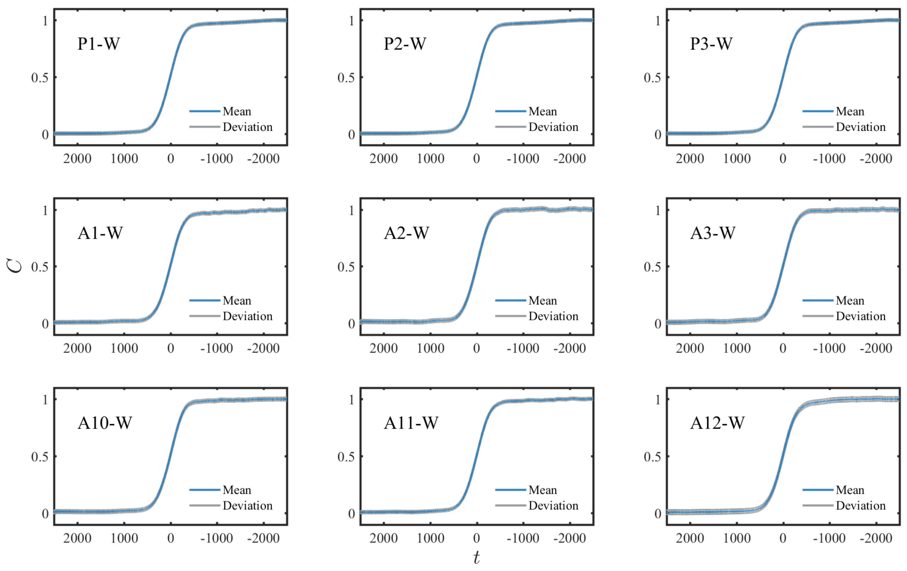
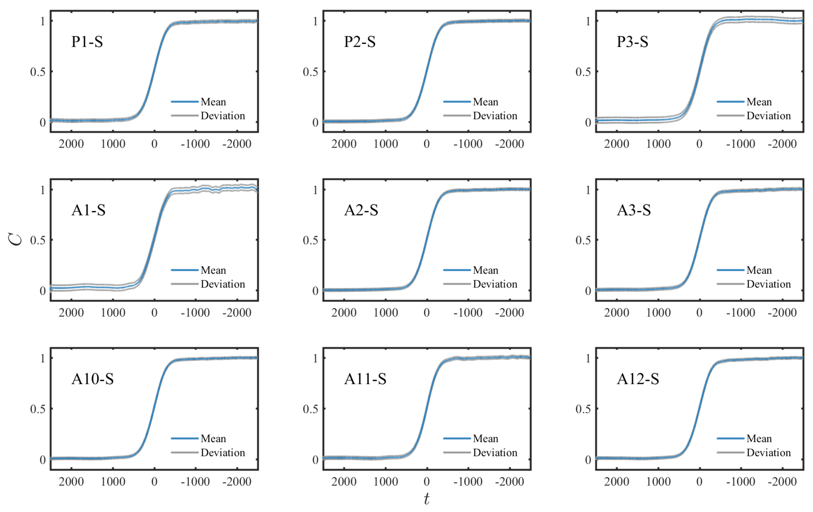
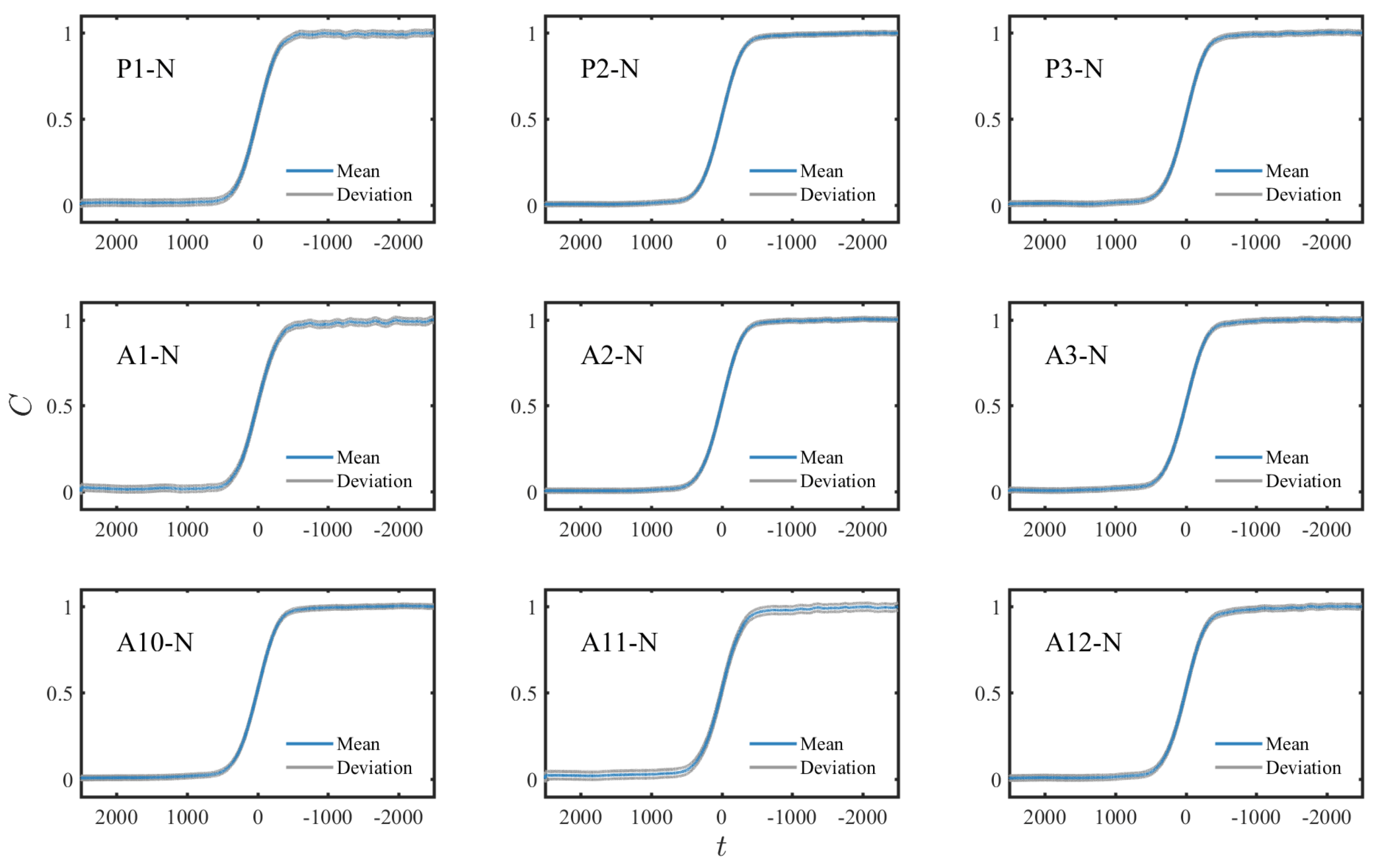
In Figure 6, we plot the BTCs measured in the east branch at the nine locations for the five repeated experiments (FN, Q10). The blue line is the average concentration based on the five repetitions and the gray lines indicate one standard deviation of the concentration of all five replicates.
The deviation at any YY fracture intersection on any Z branch is defined as:
where is the concentration of run i with , N is the total number of repeated experiments (in our study ) and is the mean of the concentration at time t, i.e.
The average deviation () for each measuring location () is defined as:
where T is the total dimensionless time of the experiment. The result (Figure 6) shows low variations between the repeated measurements which lead to small average deviations, thus implying a high confidence in our data. Corresponding data for the west, south and north branches at the nine measuring points are plotted in Appendix A (Figure A1, Figure A2, Figure A3).
3.2. Behavior across a Range of Flow Rates
We conducted 10 experiments with five unique flow rates (Table 4). The corresponding average arrival time () at the P1 location for these experiments are listed in Table 4. We observe predictable differences when flow rate is changed. However, these differences in do not perfectly correlate to the associated changes in fluid velocity and vary substantially for a given flow rate between the MFN and FN models.
As described above, this time difference is associated with the disparity in the volumes of the exterior tubing system and the micromodel interior space, such that a small variation in the starting location of the fluorescent dye in the exterior tubing can cause a large discrepancy in arrival time of the tracer. Thus, time normalization (Equation (9)) is used to bring all the data to the same temporal scale. The setup can be further improved by reducing the length of the exterior tubing and/or fabricating microfluidic valves inside the micromodel.
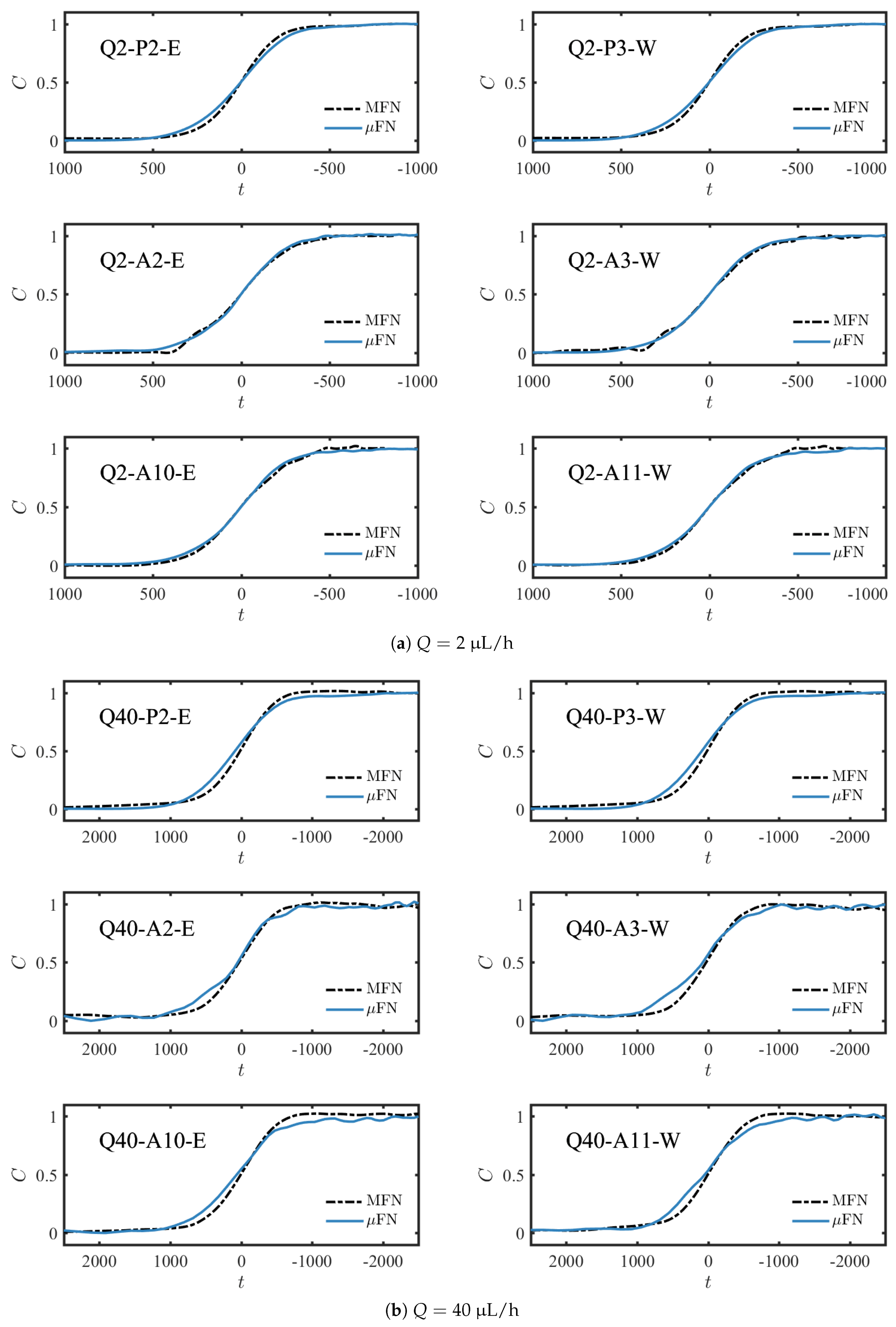
Experiments were done at five unique flow rates; the corresponding five Péclet numbers () are presented in Table 4. The Péclet number is defined as
where the length scale L is chosen as the width of the main fracture, i.e., m. Differences in the behavior of the MFN and FN models are compared using BTCs measured at common locations. The locations are selected in pairs: P2-E with P3-W, A2-E with A3-E and A10-E with A11-W. The two locations within a pair are on the same size fracture: one at the upstream end (e.g., P2-E) and the other at the downstream (e.g., P3-W) end with respect to the principle direction of flow. The space in between these two locations is a solid wall in the MFN model and has 1 m microfractures in the FN model. Therefore, this setup has the ability to quantify the influence of fracture length scale (b), transport regime () and the effect of the smallest fracture set.
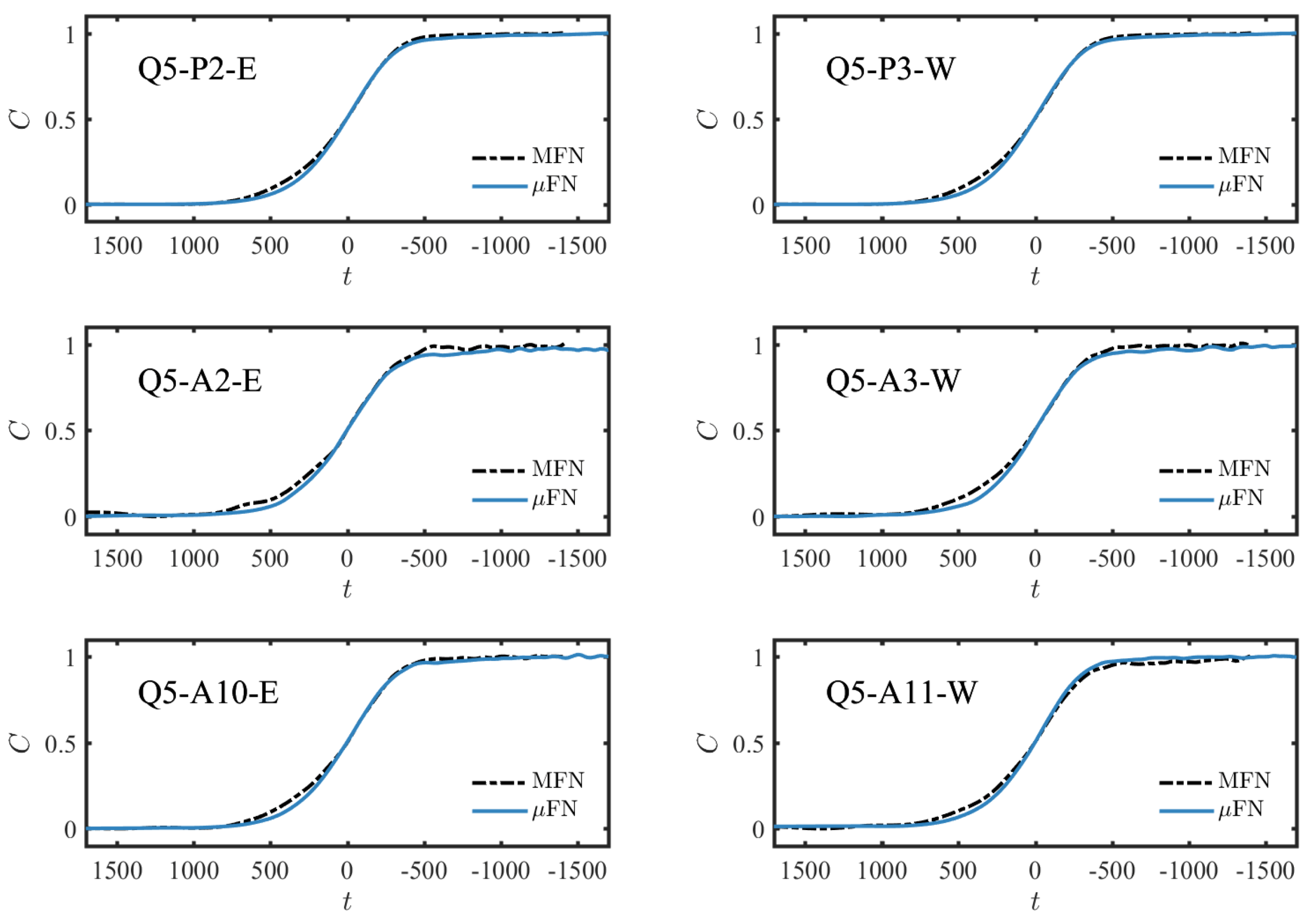
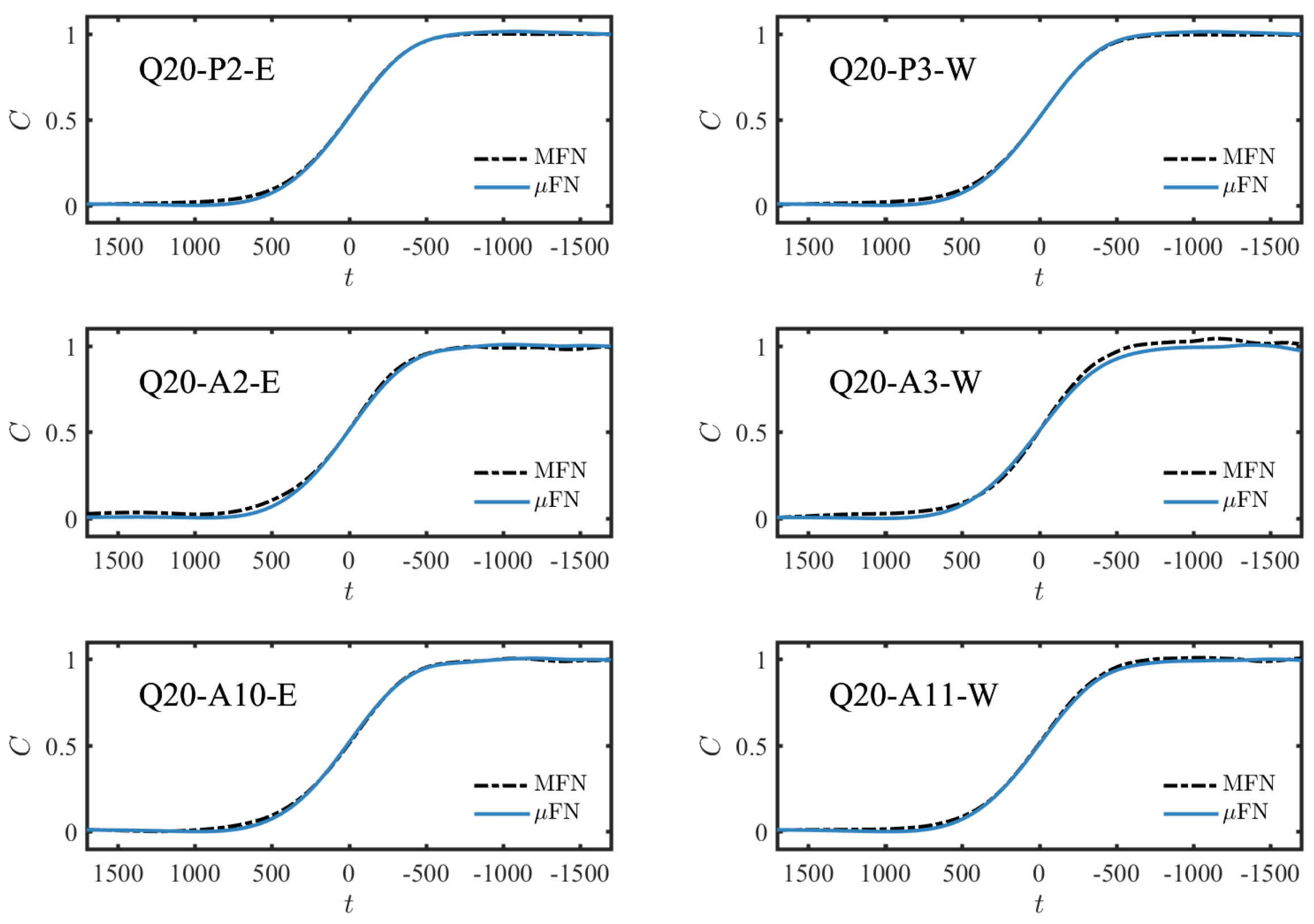
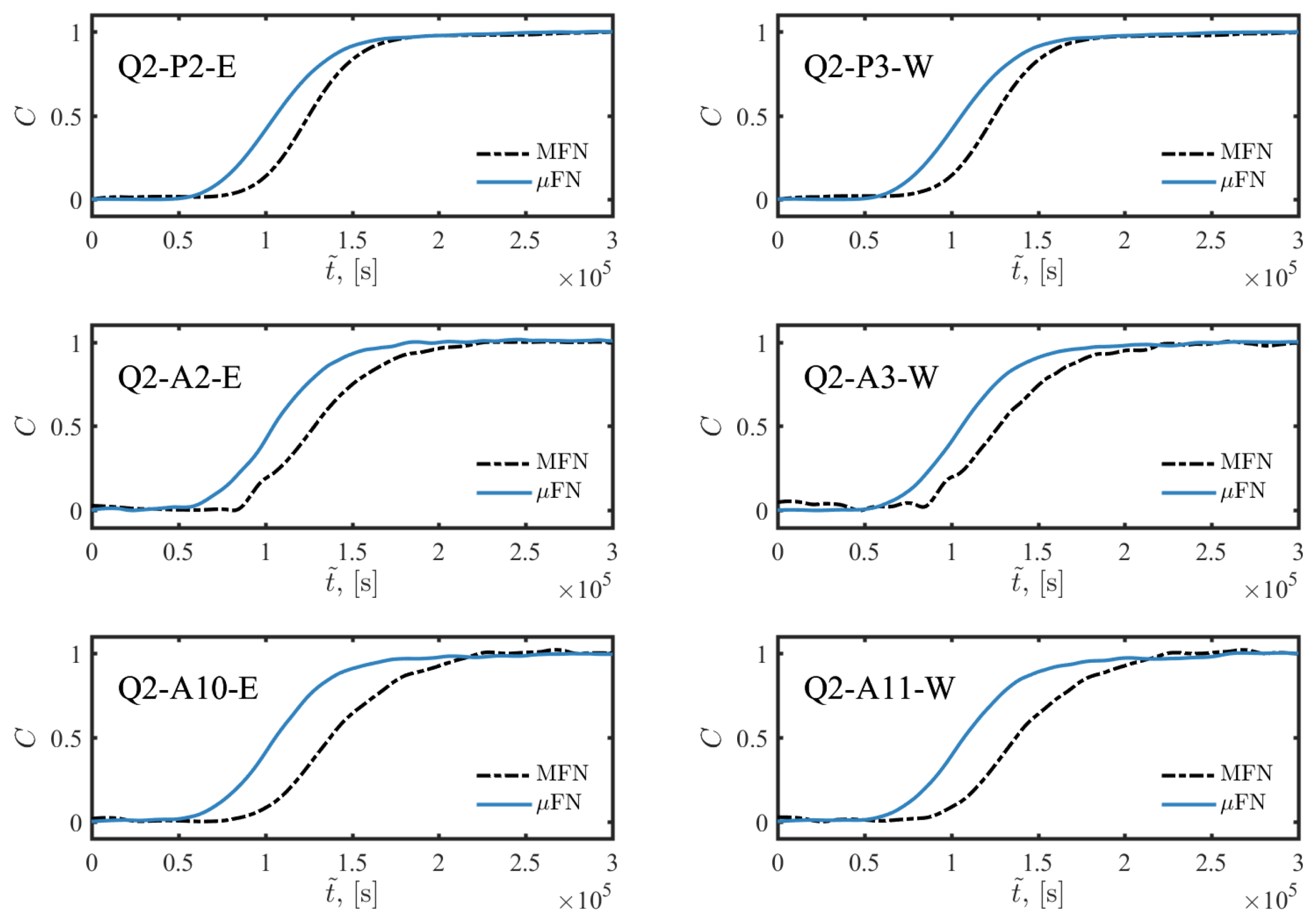
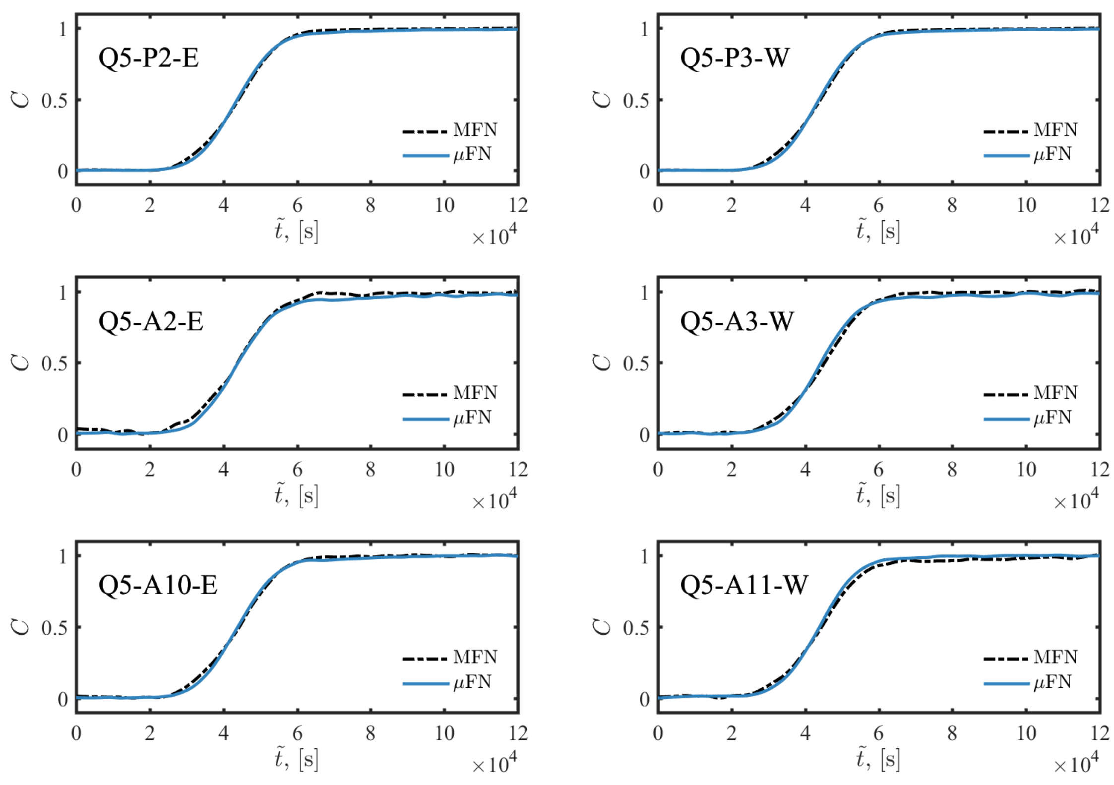
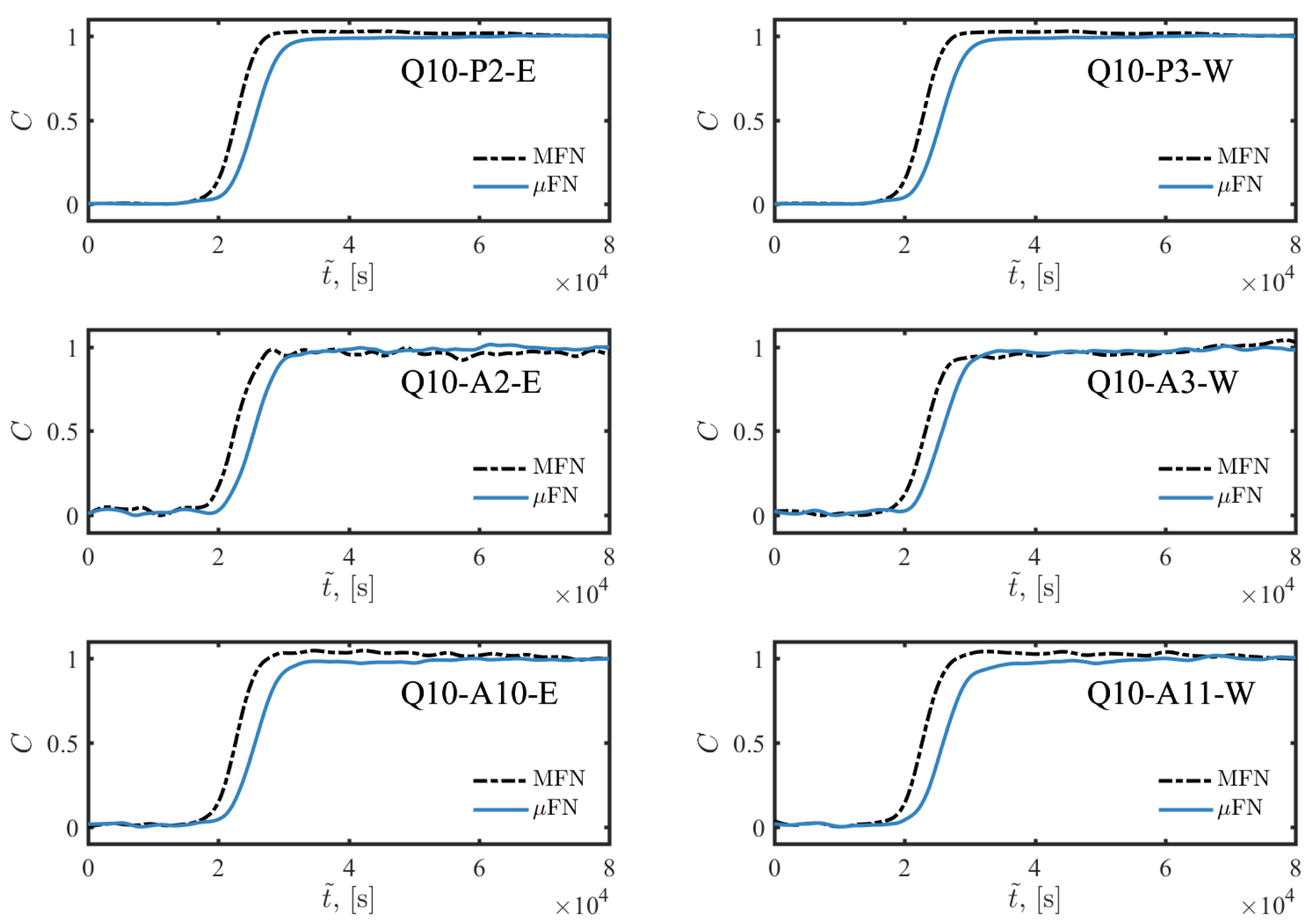
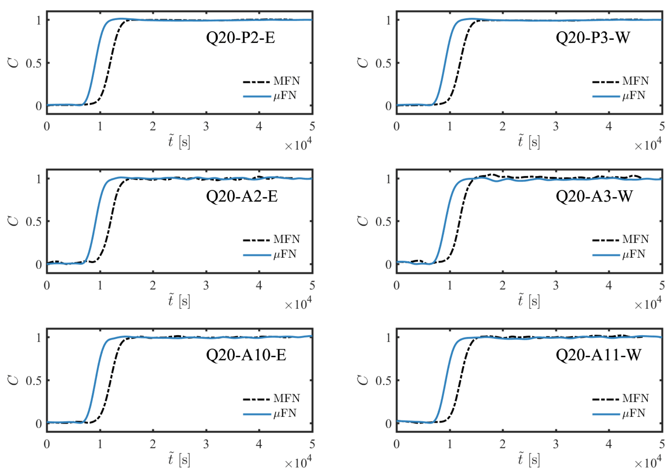
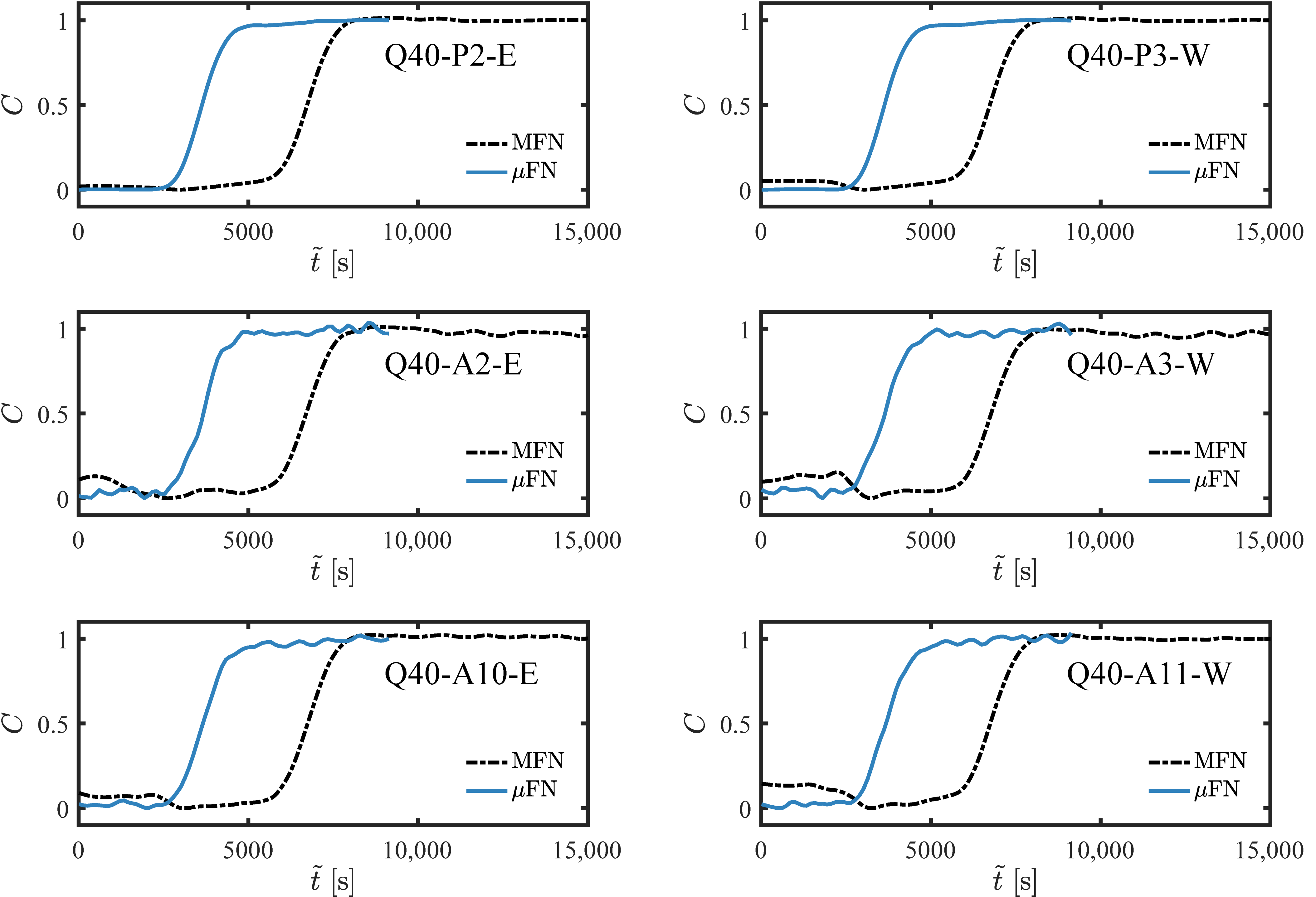
Figure 7 illustrates the results for flow rates and L/h. Additional results for other flow rates are shown in Appendix B (Figure A4, Figure A5, Figure A6) with normalized time, and results of all flow rates with physical time are shown in Figure A7, Figure A8, Figure A9, Figure A10, Figure A11. In each figure, the subplots in the left and right columns represent the BTCs at the upstream (E) and downstream (W) locations, and the dashed and solid curves are the BTCs in the MFN and the FN, respectively. Overall, the differences between the BTCs in the MFN and FN when (i.e., L/h) are larger than those at (i.e., L/h). For both and , the differences in BTCs between the two chips are smaller in fractures larger than 10 m. The smaller fractures ( and m) show difference between the MFN and the FN in both the arrival and tail of the tracer (), particularly as increases. Notably, the arrival and approach to of the tracer in the FN are generally more disperse than that of the MFN at , and this behavior appears to be most pronounced in the A2–A3 and A10–A11 secondary and tertiary fracture pairs. In the FN model, the smaller fracture apertures are quite close to the scale of the smallest microfractures, thus the impact on solute transport induced by the microfracture may be proportionally more significant, particularly at high flow rates (see Figure 7).
4. Discussion
In this study, we present the design of the first Darcy-scale microfluidic model which directly incorporates multiple orders of magnitude in length scales necessary to describe natural shale fracture patterns. To preserve the natural formation’s scaling properties, we determine the number and size of fractures based on the power law relationship observed in the field. The disparity of length scales included in the design, spanning fracture apertures between 1 and 500 m and fracture lengths between 20 and 100 mm, poses significant challenges during fabrication, flow-through system design and execution. Our results show that such challenges can be mitigated to achieve reproducible BTCs through careful design and fabrication of the micromodel, implementation of injection conditions, imaging and post-processing.
The first major challenge is the need to resolve both micro-features (1 m) and macro-features (10–500 m) with a common vertical wall height. The fabrication method must be chosen to match the applicability of a specific micro-manufacturing technique with the need to resolve the severe multi-scale nature of our micromodel. Etching methods (e.g., laser etching) are unsuitable for this application due to the non-uniformity of exposure energy. This leads to imperfect verticality of the features such that the walls between the smallest features may merge at different elevations. Soft-lithography, where the features are built using photosensitive resist and translated from a mask to a PDMS micromodel using a mold: (i) ensures high verticality of features of different sizes; and (ii) allows efficient fabrication of replicas from the same design. However, the softness of the PDMS requires an optimization of the aspect ratio between the feature size and the depth of the micromodel to prevent collapse. Furthermore, the fabrication process involves multiple steps with a lot of controllable fabrication parameters which may lead to difficulties in optimization. Here, we adopted a fabrication protocol and only varied the photo-resist composition ratio to obtain the optimal feature height in the multi-scale micromodels. In comparison with existing fabrication protocols [39,43,44], our approach shows advantages in fine tuning the feature height and provides a new fabrication control parameter in lithography applications.
The multi-scale nature of the designs also introduced challenges during the fluid injection phase. Smooth switching between different injections stages is crucial to minimize any perturbation to the flow field. Traditional switching valves are often hand operated [35,37,45] leading to large fluctuations in the flow field. We overcame this issue by utilizing electrical circuit controlled servo-motors that switch valves swiftly, simultaneously and smoothly. The enforcement of boundary conditions must also be treated with care. While no-flow conditions can be easily implemented by closing the outlets, constant pressure conditions require that the outlet ports be connected to a waste bottle through water-saturated tubes. This setup circumvents the occurrence of variable pressure conditions at the outlets, which can occur if they are left directly open to the atmosphere due to the formation of menisci of different curvatures. The setup not only provides rigorous and reproducible experimental conditions, but also strict compatibility with theoretical/numerical modeling requirements.
Additional challenges emerged during the imaging and visualization steps. A point of contention is the need for zoomed-in views to fully resolve fine-scale features and the large fields of view to capture the full multi-scale nature of the process. A balance between the two was achieved by using multi-point measurements across the chip, where the stage was moved. However, the physical distance between the measuring points across the micromodel led to significant nonuniformity in the measured light intensity, image focusing conditions, and background noise [36,40]. These effects were addressed by applying a point-wise correction to the measured intensity using the variations of the light intensity on the solid walls immediately adjacent to each measurement location. Multi-point measurements, paired with localized image correction, show good data quality with low fluctuation. While all the experiments were performed with a single diluted fluorescent dye (Alexa-488 in DI water), we expect this protocol to be applicable for similar fluid/solute combinations.
Finally, to test the robustness of the protocol as to pertains to experimental reproducibility, we also quantified experimental error through repeated runs, and we offer a normalization procedure to circumvent the discrepancy in arrival times between these replicates. Overall, this study presents the first systematic protocol for designing, fabricating and conducting multi-scale microfluidic experiments which encapsulate characteristic length scales spanning 4–5 orders of magnitude.
5. Conclusions
Natural shale rocks exhibit a power-law distribution between fracture aperture and density, such that the finest features are ubiquitous in the shale fabric. The multi-scale nature of these features can be severe as they span many orders of magnitude in sizes (both aperture and length). The overall impact on transport of such microfractures is still unknown, and thus critical to quantifying and constructing appropriate numerical modeling schemes. In this paper, we develop a protocol to physically model multi-scale fracture networks in the context of microfluidics to assess the impact of fine features and provide experimental benchmarks for systems with a large disparity of scales. The design includes two microchips (MFN and FN) with a shared backbone of primary, secondary and tertiary fractures (with apertures ranging between 5 and 500 m); FN has additional 1 m fractures superimposed at a bearing of 55°.
Such a multi-scale design requires a careful process of protocol optimization (from fabrication to image processing) to find the balance between the accuracy of resolution and repeatability of measurements across the macroscale chip. From a fabrication standpoint, optimization of the micromodel geometry (i.e., depth) is necessary to ensure accuracy in resolving the small feature topology and to prevent microchip collapse using a complex and multi-step fabrication process. To improve fluid injection and minimize the fluctuations induced by the exterior tubing, electronically-controlled fluid switches must be employed. Furthermore, employing a micromodel designed with multiple inlet/outlet ports allows the flexibility to modify boundary conditions such that they represent different injections scenarios.
In addition to the improvements in the experimental design, localized multi-point correction is necessary and practically feasible to account for the local variations in light intensity which can arise due to the physical size of the chip. With these protocols in place, repeated experimental runs have demonstrated reproducibility of results/BTCs at all scales.
This study lays the groundwork for further analysis of multi-scale systems in microfluidic models, where precisely controlled geometry can be used to systematically study the impact of topology and scale-separation on passive and reactive transport in shale fabric. The high degree of reproducibility shown in these experiments makes them perfect candidates for benchmarking new multi-scale algorithms, when the ‘tyranny of scales’ prevents and/or limits the availability of numerical pore-scale benchmarks. The multi-scale nature of the proposed design pushes the boundaries of this technology to demonstrate its full capabilities. Additional components of the experimental design, for example the ability to functionalize the PDMS surface to simulate shales surface reactivity, warrant further investigation and represent an avenue for future research.
Author Contributions
Conceptualization, B.L., I.B. and J.L.D.; methodology, B.L.; investigation, B.L. and H.J.K.; resources, I.B. and J.L.D.; data, B.L. and H.J.K.; writing—original draft preparation, B.L. and H.J.K.; and writing—review and editing, I.B. and J.L.D. All authors have read and agreed to the published version of the manuscript.
Funding
This research was funded by the Center for Mechanistic Control of Water-Hydrocarbon-Rock Interactions in Unconventional and Tight Oil Formations (CMC-UF), an Energy Frontier Research Center funded by the U.S. Department of Energy, Office of Science under DOE (BES) Award DE-SC0019165.
Acknowledgments
The authors thank Anthony Kovscek for his valuable input.
Conflicts of Interest
The authors declare no conflict of interest.
Abbreviations
The following abbreviations are used in this manuscript:
| FN | Microfracture Network |
| b | Fracture width, m |
| Background | |
| C | Dye concentration, [] |
| I | Light intensity |
| Q | Flow rate, L/h |
| BTC | Breakthrough Curve |
| DI water | De-ionized water |
| MFN | Macrofracture Network |
| PDMS | Polydimethylsiloxane |
| Péclet number |
Appendix A. Concentration Uncertainty Quantification
Figure A1.
Experimental error estimate for five repeated runs. The blue curve is the mean of the experiments that measured at the west (W) branch at each location and the gray curve is the average deviation.
Figure A1.
Experimental error estimate for five repeated runs. The blue curve is the mean of the experiments that measured at the west (W) branch at each location and the gray curve is the average deviation.

Figure A2.
Experimental error estimate for five repeated runs. The blue curve is the mean of the experiments that measured at the south (S) branch at each location and the gray curve is the average deviation.
Figure A2.
Experimental error estimate for five repeated runs. The blue curve is the mean of the experiments that measured at the south (S) branch at each location and the gray curve is the average deviation.

Figure A3.
Experimental error estimate for five repeated runs. The blue curve is the mean of the experiments that measured at the north (N) branch at each location and the gray curve is the average deviation.
Figure A3.
Experimental error estimate for five repeated runs. The blue curve is the mean of the experiments that measured at the north (N) branch at each location and the gray curve is the average deviation.

Appendix B. Upper Stream and Down Stream BTCs with Normalized Time
Figure A4.
Measured breakthrough curves in the MFN (dashed line) and FN (solid line) at upstream (east) and downstream (west) locations on the same primary (P2–P3), secondary (A10–A11) and tertiary (A2–A3) fracture at L/h.
Figure A4.
Measured breakthrough curves in the MFN (dashed line) and FN (solid line) at upstream (east) and downstream (west) locations on the same primary (P2–P3), secondary (A10–A11) and tertiary (A2–A3) fracture at L/h.

Figure A5.
Measured breakthrough curves in the MFN (dashed line) and FN (solid line) at upstream (east) and downstream (west) locations on the same primary (P2–P3), secondary (A10–A11) and tertiary (A2–A3) fracture at L/h.
Figure A5.
Measured breakthrough curves in the MFN (dashed line) and FN (solid line) at upstream (east) and downstream (west) locations on the same primary (P2–P3), secondary (A10–A11) and tertiary (A2–A3) fracture at L/h.

Figure A6.
Measured breakthrough curves in the MFN (dashed line) and FN (solid line) at upstream (east) and downstream (west) locations on the same primary (P2–P3), secondary (A10–A11) and tertiary (A2–A3) fracture at L/h.
Figure A6.
Measured breakthrough curves in the MFN (dashed line) and FN (solid line) at upstream (east) and downstream (west) locations on the same primary (P2–P3), secondary (A10–A11) and tertiary (A2–A3) fracture at L/h.

Appendix C. BTC with Physical Time
Figure A7.
Breakthrough curves measured in physical time in the MFN (dashed line) and FN (solid line) at upstream (east) and downstream (west) locations on the same primary (P2–P3), secondary (A10–A11) and tertiary (A2–A3) fracture at L/h.
Figure A7.
Breakthrough curves measured in physical time in the MFN (dashed line) and FN (solid line) at upstream (east) and downstream (west) locations on the same primary (P2–P3), secondary (A10–A11) and tertiary (A2–A3) fracture at L/h.

Figure A8.
Breakthrough curves measured in physical time in the MFN (dashed line) and FN (solid line) at upstream (east) and downstream (west) locations on the same primary (P2–P3), secondary (A10–A11) and tertiary (A2–A3) fracture at L/h.
Figure A8.
Breakthrough curves measured in physical time in the MFN (dashed line) and FN (solid line) at upstream (east) and downstream (west) locations on the same primary (P2–P3), secondary (A10–A11) and tertiary (A2–A3) fracture at L/h.

Figure A9.
Breakthrough curves measured in physical time in the MFN (dashed line) and FN (solid line) at upstream (east) and downstream (west) locations on the same primary (P2–P3), secondary (A10–A11) and tertiary (A2–A3) fracture at L/h.
Figure A9.
Breakthrough curves measured in physical time in the MFN (dashed line) and FN (solid line) at upstream (east) and downstream (west) locations on the same primary (P2–P3), secondary (A10–A11) and tertiary (A2–A3) fracture at L/h.

Figure A10.
Breakthrough curves measured in physical time in the MFN (dashed line) and FN (solid line) at upstream (east) and downstream (west) locations on the same primary (P2–P3), secondary (A10–A11) and tertiary (A2–A3) fracture at L/h.
Figure A10.
Breakthrough curves measured in physical time in the MFN (dashed line) and FN (solid line) at upstream (east) and downstream (west) locations on the same primary (P2–P3), secondary (A10–A11) and tertiary (A2–A3) fracture at L/h.

Figure A11.
Breakthrough curves measured in physical time in the MFN (dashed line) and FN (solid line) at upstream (east) and downstream (west) locations on the same primary (P2–P3), secondary (A10–A11) and tertiary (A2–A3) fracture at L/h.
Figure A11.
Breakthrough curves measured in physical time in the MFN (dashed line) and FN (solid line) at upstream (east) and downstream (west) locations on the same primary (P2–P3), secondary (A10–A11) and tertiary (A2–A3) fracture at L/h.

References
- US Energy Information Administration. Annual Energy Outlook 2019 with Projections to 2050; Technical Report; US Energy Information Administration: Washington, DC, USA, 2019.
- Wood, D.A.; Hazra, B. Characterization of organic-rich shales for petroleum exploration & exploitation: A review-Part 1: Bulk properties, multi-scale geometry and gas adsorption. J. Earth Sci. 2017, 28, 758–778. [Google Scholar]
- Gensterblum, Y.; Ghanizadeh, A.; Cuss, R.J.; Amann-Hildenbrand, A.; Krooss, B.M.; Clarkson, C.R.; Harrington, J.F.; Zoback, M.D. Gas transport and storage capacity in shale gas reservoirs–A review. Part A: Transport processes. J. Unconv. Oil Gas Resour. 2015, 12, 87–122. [Google Scholar] [CrossRef]
- Wu, W.; Sharma, M.M. Acid Fracturing in Shales: Effect of Dilute Acid on Properties and Pore Structure of Shale. SPE Prod. Oper. 2017, 32, 51–63. [Google Scholar] [CrossRef]
- Javadpour, F.; Fisher, D.; Unsworth, M. Nanoscale Gas Flow in Shale Gas Sediments. J. Can. Pet. Technol. 2007, 46. [Google Scholar] [CrossRef]
- Ilgen, A.G.; Heath, J.E.; Akkutlu, I.Y.; Bryndzia, L.T.; Cole, D.R.; Kharaka, Y.K.; Kneafsey, T.J.; Milliken, K.L.; Pyrak-Nolte, L.J.; Suarez-Rivera, R. Shales at all scales: Exploring coupled processes in mudrocks. Earth-Sci. Rev. 2017, 166, 132–152. [Google Scholar] [CrossRef] [Green Version]
- Bai, B.; Elgmati, M.; Zhang, H.; Wei, M. Rock characterization of Fayetteville shale gas plays. Fuel 2013, 105, 645–652. [Google Scholar] [CrossRef]
- Clarkson, C.R.; Solano, N.; Bustin, R.M.; Bustin, A.M.M.; Chalmers, G.R.L.; He, L.; Melnichenko, Y.B.; Radliński, A.P.; Blach, T.P. Pore structure characterization of North American shale gas reservoirs using USANS/SANS, gas adsorption, and mercury intrusion. Fuel 2013, 103, 606–616. [Google Scholar] [CrossRef]
- King, H.E.; Eberle, A.P.R.; Walters, C.C.; Kliewer, C.E.; Ertas, D.; Huynh, C. Pore Architecture and Connectivity in Gas Shale. Energy Fuels 2015, 29, 1375–1390. [Google Scholar] [CrossRef]
- Vishal, V.; Chandra, D.; Bahadur, J.; Sen, D.; Hazra, B.; Mahanta, B.; Mani, D. Interpreting Pore Dimensions in Gas Shales Using a Combination of SEM Imaging, Small-Angle Neutron Scattering, and Low-Pressure Gas Adsorption. Energy Fuels 2019, 33, 4835–4848. [Google Scholar] [CrossRef]
- Zhang, Y.; Barber, T.J.; Hu, Q.; Bleuel, M.; El-Sobky, H.F. Complementary neutron scattering, mercury intrusion and SEM imaging approaches to micro- and nano-pore structure characterization of tight rocks: A case study of the Bakken shale. Int. J. Coal Geol. 2019, 212, 103252. [Google Scholar] [CrossRef]
- Frouté, L.; Kovscek, A.R. Nano-Imaging of Shale Using Electron Microscopy Techniques. In Proceedings of the Unconventional Resources Technology Conference (URTeC), Virtual, 20–22 July 2020. [Google Scholar] [CrossRef]
- Lee, K.S.; Kim, T.H. Transport in Shale Reservoirs; Gulf Professional Publishing: Cambridge, MA, USA, 2019. [Google Scholar]
- Gale, J.F.W.; Laubach, S.E.; Olson, J.E.; Eichhubl, P.; Fall, A. Natural fractures in shale: A review and new observations. AAPG Bull. 2014, 98, 2165–2216. [Google Scholar] [CrossRef]
- Wang, Q.; Gale, J.F. Characterizing Bedding-Parallel Fractures in Shale: Aperture-Size Distributions and Spatial Organization. In Proceedings of the 2016 AAPG Annual Convention and Exhibition, Calgary, AB, Canada, 19–22 June 2016. [Google Scholar]
- Mi, L.; Jiang, H.; Li, J.; Li, T.; Tian, Y. The investigation of fracture aperture effect on shale gas transport using discrete fracture model. J. Nat. Gas Sci. Eng. 2014, 21, 631–635. [Google Scholar] [CrossRef]
- Li, Q.; Xing, H.; Liu, J.; Liu, X. A review on hydraulic fracturing of unconventional reservoir. Petroleum 2015, 1, 8–15. [Google Scholar] [CrossRef] [Green Version]
- Harrison, A.L.; Jew, A.D.; Dustin, M.K.; Thomas, D.L.; Joe-Wong, C.M.; Bargar, J.R.; Johnson, N.; Brown, G.E.; Maher, K. Element release and reaction-induced porosity alteration during shale-hydraulic fracturing fluid interactions. Appl. Geochem. 2017, 82, 47–62. [Google Scholar] [CrossRef]
- Balashov, V.N.; Guthrie, G.D.; Lopano, C.L.; Hakala, J.A.; Brantley, S.L. Reaction and diffusion at the reservoir/shale interface during CO2 storage: Impact of geochemical kinetics. Appl. Geochem. 2015, 61, 119–131. [Google Scholar] [CrossRef]
- Hakala, J.A.; Crandall, D.; Moore, J.; Phan, T.; Sharma, S.; Lopano, C. Laboratory-Scale Studies on Chemical Reactions Between Fracturing Fluid and Shale Core From the Marcellus Shale Energy and Environmental Laboratory (MSEEL) Site. In Proceedings of the Unconventional Resources Technology Conference, Austin, TX, USA, 24–26 July 2017. [Google Scholar] [CrossRef] [Green Version]
- Dahi Taleghani, A.; Olson, J.E. How Natural Fractures Could Affect Hydraulic-Fracture Geometry. SPE J. 2013, 19, 161–171. [Google Scholar] [CrossRef]
- Wu, K.; Olson, J.E. Mechanics Analysis of Interaction Between Hydraulic and Natural Fractures in Shale Reservoirs. In Proceedings of the Unconventional Resources Technology Conference, Denver, CO, USA, 25–27 August 2014. [Google Scholar] [CrossRef]
- Kolawole, O.; Ispas, I. Interaction between hydraulic fractures and natural fractures: Current status and prospective directions. J. Pet. Explor. Prod. Technol. 2020, 10, 1613–1634. [Google Scholar] [CrossRef] [Green Version]
- Shrivastava, K.; Sharma, M.M. Mechanisms for the Formation of Complex Fracture Networks in Naturally Fractured Rocks; Society of Petroleum Engineers: Richardson, TX, USA, 2018. [Google Scholar] [CrossRef]
- Saif, T.; Lin, Q.; Butcher, A.R.; Bijeljic, B.; Blunt, M.J. Multi-scale multi-dimensional microstructure imaging of oil shale pyrolysis using X-ray micro-tomography, automated ultra-high resolution SEM, MAPS Mineralogy and FIB-SEM. Appl. Energy 2017, 202, 628–647. [Google Scholar] [CrossRef]
- Wang, H.; Chen, L.; Qu, Z.; Yin, Y.; Kang, Q.; Yu, B.; Tao, W.Q. Modeling of multi-scale transport phenomena in shale gas production—A critical review. Appl. Energy 2020, 262, 114575. [Google Scholar] [CrossRef]
- Tsang, C.F. Tracer Transport in Fracture Systems. In Flow and Contaminant Transport in Fractured Rock; Bear, J., Tsang, C.F., de Marsily, G., Eds.; Academic Press: Oxford, UK, 1993; pp. 237–266. [Google Scholar] [CrossRef]
- Bodin, J.; Delay, F.; de Marsily, G. Solute transport in a single fracture with negligible matrix permeability: 1. fundamental mechanisms. Hydrogeol. J. 2003, 11, 418–433. [Google Scholar] [CrossRef]
- Kosakowski, G.; Berkowitz, B. Flow pattern variability in natural fracture intersections. Geophys. Res. Lett. 1999, 26, 1765–1768. [Google Scholar] [CrossRef]
- Zhao, Z.; Li, B.; Jiang, Y. Effects of Fracture Surface Roughness on Macroscopic Fluid Flow and Solute Transport in Fracture Networks. Rock Mech. Rock Eng. 2014, 47, 2279–2286. [Google Scholar] [CrossRef]
- Zou, L.; Jing, L.; Cvetkovic, V. Modeling of Solute Transport in a 3D Rough-Walled Fracture-Matrix System. Transp. Porous Media 2017, 116, 1005–1029. [Google Scholar] [CrossRef] [Green Version]
- Charlet, L.; Alt-Epping, P.; Wersin, P.; Gilbert, B. Diffusive transport and reaction in clay rocks: A storage (nuclear waste, CO2, H2), energy (shale gas) and water quality issue. Adv. Water Resour. 2017, 106, 39–59. [Google Scholar] [CrossRef] [Green Version]
- Graf, T.; Therrien, R. Variable-density groundwater flow and solute transport in irregular 2D fracture networks. Adv. Water Resour. 2007, 30, 455–468. [Google Scholar] [CrossRef]
- Field, M.S. On Tracer Breakthrough Curve Dataset Size, Shape, and Statistical Distribution. Adv. Water Resour. 2020, 141, 103596. [Google Scholar] [CrossRef]
- Zhang, C.; Oostrom, M.; Wietsma, T.W.; Grate, J.W.; Warner, M.G. Influence of viscous and capillary forces on immiscible fluid displacement: Pore-scale experimental study in a water-wet micromodel demonstrating viscous and capillary fingering. Energy Fuels 2011, 25, 3493–3505. [Google Scholar] [CrossRef]
- Werth, C.J.; Zhang, C.; Brusseau, M.L.; Oostrom, M.; Baumann, T. A review of non-invasive imaging methods and applications in contaminant hydrogeology research. J. Contam. Hydrol. 2010, 113, 1–24. [Google Scholar] [CrossRef] [Green Version]
- Ling, B.; Oostrom, M.; Tartakovsky, A.M.; Battiato, I. Hydrodynamic dispersion in thin channels with micro-structured porous walls. Phys. Fluids 2018, 30, 076601. [Google Scholar] [CrossRef]
- Karadimitriou, N.; Hassanizadeh, S. A review of micromodels and their use in two-phase flow studies. Vadose Zone J. 2012, 11. [Google Scholar] [CrossRef]
- Xia, Y.; Whitesides, G.M. Soft lithography. Ann. Rev. Mater. Sci. 1998, 28, 153–184. [Google Scholar] [CrossRef]
- Willingham, T.W.; Werth, C.J.; Valocchi, A.J. Evaluation of the effects of porous media structure on mixing-controlled reactions using pore-scale modeling and micromodel experiments. Environ. Sci. Technol. 2008, 42, 3185–3193. [Google Scholar] [CrossRef] [PubMed]
- Aljamaan, H.; Ross, C.M.; Kovscek, A.R. Multiscale Imaging of Gas Storage in Shales. SPE J. 2017, 22, 1760–1777. [Google Scholar] [CrossRef]
- Ogata, A.; Banks, R.B. A Solution of the Differential Equation of Longitudinal Dispersion in Porous Media; US Government Printing Office: Washington, DC, USA, 1961.
- Folch, A.; Ayon, A.; Hurtado, O.; Schmidt, M.; Toner, M. Molding of deep polydimethylsiloxane microstructures for microfluidics and biological applications. J. Biomech. Eng. 1999, 121, 28–34. [Google Scholar] [CrossRef] [Green Version]
- Kim, P.; Kwon, K.W.; Park, M.C.; Lee, S.H.; Kim, S.M.; Suh, K.Y. Soft lithography for microfluidics: A review. Biochip J. 2008, 2, 1–11. [Google Scholar]
- Ling, B.; Bao, J.; Oostrom, M.; Battiato, I.; Tartakovsky, A.M. Modeling variability in porescale multiphase flow experiments. Adv. Water Resour. 2017, 105, 29–38. [Google Scholar] [CrossRef]
Figure 1.
Scaling relationship between fracture aperture (b) and frequency (f). Marcellus shale experimental data is reproduced from [14].
Figure 1.
Scaling relationship between fracture aperture (b) and frequency (f). Marcellus shale experimental data is reproduced from [14].

Figure 2.
Two fracture networks are designed for this study: the MFN (left) contains fractures with apertures within 5–500 m and the FN (right) is characterized by the same backbone of the MFN with the addition of 119 1 m fractures. The circular markers on the rim of the fracture networks are inlet (red) and outlet (blue) ports.

Figure 3.
Experimental setup: (A) injection and tubing system; (B) injection patterns; and imaging system and photograph of actual setup.
Figure 3.
Experimental setup: (A) injection and tubing system; (B) injection patterns; and imaging system and photograph of actual setup.

Figure 4.
(A) Nine measuring locations (black boxes) and definition of fracture branches; and (B) actual microscopy images with water-saturated (left) and solute-saturated (right) fractures.
Figure 4.
(A) Nine measuring locations (black boxes) and definition of fracture branches; and (B) actual microscopy images with water-saturated (left) and solute-saturated (right) fractures.

Figure 5.
(Top) Measured light intensity (, solid line) at location A1-E of the FN for L/h and measured background measurement (, dashed line) next to A1-E; (Middle) normalized concentration as a function of physical time (); and (Bottom) normalized concentration as a function of normalized time (t).

Figure 6.
Experimental error estimate for five repeated runs. The blue curve is the mean of the experiments and the gray curve is the average deviation.
Figure 6.
Experimental error estimate for five repeated runs. The blue curve is the mean of the experiments and the gray curve is the average deviation.

Figure 7.
Measured BTCs in the MFN (dashed line) and FN (solid line) at upstream (east) and downstream (west) locations on the same primary (P2–P3), secondary (A10–A11) and tertiary (A2–A3) fracture at: (a) L/h; and (b) L/h.
Figure 7.
Measured BTCs in the MFN (dashed line) and FN (solid line) at upstream (east) and downstream (west) locations on the same primary (P2–P3), secondary (A10–A11) and tertiary (A2–A3) fracture at: (a) L/h; and (b) L/h.


Table 1.
Number of fractures contained in the MFN and FN micromodels.
| Fracture Number | ||
|---|---|---|
| Aperture | MFN | FN |
| 500 m | 1 | 1 |
| 20 m | 2 | 2 |
| 10 m | 6 | 6 |
| 5 m | 14 | 14 |
| 1 m | 0 | 119 |
Table 2.
Coordinates of imaged intersections.
| Location | x-Coordinate (mm) | y-Coordinate (mm) | Horizontal Fracture (m) | Vertical Fracture (m) |
|---|---|---|---|---|
| P1 | 11.78 | 0 | 500 | 5 |
| P2 | 16.61 | 0 | 500 | 20 |
| P3 | 26.70 | 0 | 500 | 10 |
| A1 | 12.76 | 5.20 | 5 | 5 |
| A2 | 17.98 | 5.14 | 5 | 20 |
| A3 | 28.13 | 5.02 | 5 | 10 |
| A10 | 19.73 | 11.67 | 10 | 20 |
| A11 | 23.88 | 11.67 | 10 | 5 |
| A12 | 30.03 | 11.67 | 10 | 10 |
Table 3.
Properties and experimental parameters.
| Symbol | Value | Unit | |
|---|---|---|---|
| Main fracture width | B | 500 | m |
| Main fracture length | L | 70 | mm |
| fracture network thickness | 10 | m | |
| Fluid density | 1000 | kg/m | |
| Fluid kinetic viscosity | m/s | ||
| Solute molecular diffusivity | m/s | ||
| Injection flow rate | Q | 2–40 | L/h |
| Average inlet velocity | 2.7–21.6 | m/s |
Table 4.
Experiment flow rates, Péclet number and P1 arrival time.
| Label | Flow Rate (L/h) | Peclet Number (–) | P1 Arrival Time (mins) |
|---|---|---|---|
| MFN, Q2 | 2 | 124 | 2085.15 |
| FN, Q2 | 2 | 124 | 1767.19 |
| MFN, Q5 | 5 | 310 | 736.19 |
| FN, Q5 | 5 | 310 | 730.12 |
| MFN, Q10 | 10 | 620 | 378.16 |
| FN, Q10 | 10 | 620 | 426.18 |
| MFN, Q20 | 20 | 1240 | 200.20 |
| FN, Q20 | 20 | 1240 | 153.17 |
| MFN, Q40 | 40 | 2480 | 112.48 |
| FN, Q40 | 40 | 2480 | 62.14 |
| FN, Q10(R1) | 10 | 620 | 309.25 |
| FN, Q10(R2) | 10 | 620 | 391.31 |
| FN, Q10(R3) | 10 | 620 | 375.21 |
| FN, Q10(R4) | 10 | 620 | 391.26 |
Publisher’s Note: MDPI stays neutral with regard to jurisdictional claims in published maps and institutional affiliations. |
© 2020 by the authors. Licensee MDPI, Basel, Switzerland. This article is an open access article distributed under the terms and conditions of the Creative Commons Attribution (CC BY) license (http://creativecommons.org/licenses/by/4.0/).
Share and Cite
MDPI and ACS Style
Ling, B.; Khan, H.J.; Druhan, J.L.; Battiato, I. Multi-Scale Microfluidics for Transport in Shale Fabric. Energies 2021, 14, 21. https://doi.org/10.3390/en14010021
AMA Style
Ling B, Khan HJ, Druhan JL, Battiato I. Multi-Scale Microfluidics for Transport in Shale Fabric. Energies. 2021; 14(1):21. https://doi.org/10.3390/en14010021
Chicago/Turabian StyleLing, Bowen, Hasan J. Khan, Jennifer L. Druhan, and Ilenia Battiato. 2021. "Multi-Scale Microfluidics for Transport in Shale Fabric" Energies 14, no. 1: 21. https://doi.org/10.3390/en14010021
Note that from the first issue of 2016, this journal uses article numbers instead of page numbers. See further details here.