
Fractal Characterization of Multimodal, Multiscale Images of Shale Rock Fracture Networks


Department of Energy Resources Engineering, Stanford University, Stanford, CA 94305, USA
*
Author to whom correspondence should be addressed.
Energies 2022, 15(3), 1012; https://doi.org/10.3390/en15031012
Submission received: 1 December 2021
/
Revised: 15 January 2022
/
Accepted: 17 January 2022
/
Published: 29 January 2022
(This article belongs to the Special Issue Pore-Scale Multiphase Fluid Flow and Transport in Porous Media)
Abstract
:An array of multimodal and multiscale images of fractured shale rock samples and analogs was collected with the aim of improving the numerical representation of fracture networks. 2D and 3D reconstructions of fractures and matrices span from 10−6 to 100 m. The origin of the fracture networks ranged from natural to thermal maturation to hydraulically induced maturation. Images were segmented to improve fracture identification. Then, the fractal dimension and length distribution of the fracture networks were calculated for each image dataset. The resulting network connectivity and scaling associations are discussed at length on the basis of scale, sample and order of magnitude. Fracture network origin plays an important role in the resulting fracture systems and their scaling. Rock analogs are also evaluated using these descriptive tools and are found to be faithful depictions of maturation-induced fracture networks.
Keywords:
shale rock; fractal; image analysis; rock analogs; fracture network; scaling; connectivity1. Introduction
Interest in the study of unconventional rocks (shales, mudstones, siltstones, marls, etc.) has significantly increased in the last decade. Historically, shale formations were regarded as either source or seal rocks [1] while being overlooked for their energy resource potential. This drastically changed with the increase in the use of hydraulic fracturing and horizontal wells. The subsequent surge of natural gas production in the United States brought unconventional formations to the attention of the energy community. Significant research has been conducted since to study unconventional porous media and its transport properties [2,3,4,5,6,7,8,9,10].
Even though the interest in characterizing and modeling shale rock properties continues to be relevant, environmental concerns regarding the control of greenhouse gas emissions and storage have prompted research on the use of depleted shale reservoirs for CO2 storage. CO2 capture followed by immobilization within geological structures is an option with the potential to decrease carbon dioxide emissions [11]. Shale formations are sites of interest for the subsurface storage of CO2 because of their gas storage capacity within their organic matter and pore space [12,13,14,15,16]. Shale formations can also act as seals for potential subsurface hydrogen storage in conventional reservoirs [17,18].
In unconventional rocks, fracture networks are presumed to constitute especially significant pathways for fluid transport. Fracture networks are considered to play a relevant role in the flow dynamics of shale host rock [19,20]. Network connectivity in low-permeability geological formations such as shale is, therefore, a critical feature controlling fluid transport [21]. Common sources of fracture networks within shale are the product of natural geological evolution, organic matter maturation, and hydraulic stimulation, among others [22,23]. Additionally, fracture networks are expected to contribute to shale rock’s total CO2 storage capacity, in particular around areas of improved injectivity [16].
Characterizing fractured unconventional rock remains challenging. The spatial heterogeneity and complexity of fracture networks at all scales compound the difficulty of creating physically accurate fracture networks and the models of transport within those networks. The multiscale nature of fracture networks and their complex geometry make efforts to characterize them accurately and efficiently a difficult task in order to help define basic transport properties [24].
The concept of fractal geometry was first introduced by Mandelbrot [25]. It has since been explored in many fields of science. Fractal geometry helps describe objects that are difficult to characterize using Euclidean geometry at all scales. The probability distribution N of a self-similar variable a conforms to an inverse power-law distribution [26]. The transition between scales depends upon D ( fractal dimension) and the slope k of a power-law curve as [27]
Fractal shapes are by definition scale invariant and self-similar, and they are characterized by their fractal dimension. In geosciences, the physics of fracturing has been proposed to be self-similar and to follow the rules of fractal behavior. Many studies have applied fractal geometry to characterize and describe porous media and fracture patterns in natural rocks, particularly in major fault systems [28,29,30,31,32,33,34,35].
Numerous studies at various scales have shown that the distribution of some fracture properties, such as length, often follow a power-law and as such, do not exhibit a characteristic length scale. Fractal geometry has been acknowledged as a tool to characterize fractured systems [32]. Interdependence between fracture length distribution l and the fractal dimension often observed in most fracture networks may be central to determining network connectivity [21]. Several studies have used a fracture network model that delineates connectivity based on the assumption that the fracture length distribution n(l) follows a power-law with an exponent such that:
Under this model [32], if > 3 for 2D networks, then connectivity is controlled by the smallest fractures and the system responds to the basis of percolation theory. Whereas, if < 2, the large fractures dominate connectivity and transport and if 2 < < 3, both small and large fractures control the network’s connectivity [21,36]. When this model is combined with fractal density distribution, the following results emerge.
- Length distribution prevails over fractal geometry, and large fractures dominate global connectivity for:
- Connectivity is controlled by fractures much smaller than the system size when:
- The system is self-similar when the transition between regimes and connectivity properties are scale invariant as
The objective of this study was to characterize fracture networks in unconventional rock samples and their analogs by calculating fractal dimensions and fracture length distributions. The dataset consists of fractured shale rock and rock analogs. The multidimensional, multimodal, and multiscale imagery was sourced from published and unpublished data at sample scales ranging from 10−6 to 100 m. The fracture network characterization was made on the basis of fractal dimension and the fitting of fracture length distributions as power-law functions. Image processing and segmentation were performed on each image of the dataset. The relation between the calculated fractal dimension and the power-law exponent of the fracture length distribution was used to evaluate the connectivity and scaling behavior of each fracture network across six orders of magnitude of sample size length, according to the connectivity model described above. The results are discussed on the basis of image scale, dimension, and fracture network origin. Finally, the feasibility of rock analogs and microfluidic models of shale rock fracture network systems are validated.
2. Materials and Methods
2.1. Sample Image Dataset
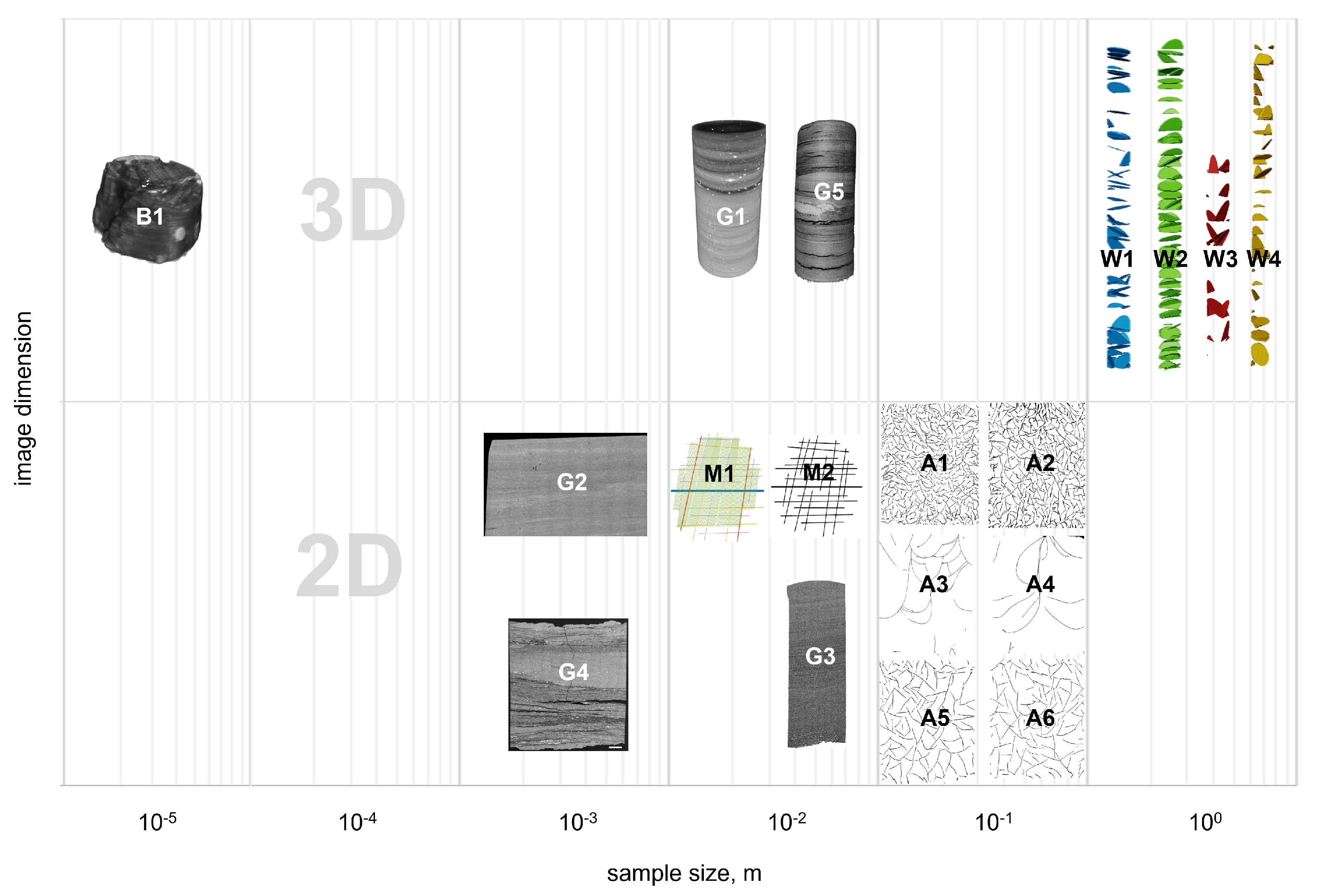
A collection of multidimensional, multimodal, and multiscale shale core sample and rock analog images with sample sizes ranging from microns to meters and resolution ranging from nanometers to microns was sourced from published [37,38,39] and our unpublished data. A visual summary of the data included in this study, sorted according to Euclidean (vertical axis) and length (horizontal axis) dimensions is shown in Figure 1. The images are otherwise not to scale. The image samples are grouped as grayscale microscopy, high-resolution photography, and tabular and graphic models according to imaging modality.
Table 1 presents a summary of the image data used in this study including scale, image resolution, imaging modality, and the origin of cracks and fractures: heat induced (HI)—via pyrolysis—or natural or fracked (N,F)). These distinctions do not technically apply to the rock analogs or models; therefore, those samples show an ‘N/A’ in that category.
Grayscale microscopy (G series): Scanning Electron Microscope (SEM) mosaics images and X-ray nano- and micro-tomography reconstructions of samples from the Green River formation were sourced from [37,40]. High-resolution photography (A series): These are images of rock analog materials at the meso-scale (lab-grade gelatin), acquired with a high-resolution DSLR camera in a setup and process described in [38]. Tabular and graphic (W series): Macro-scale fracture networks were generated from tabular fracture data reported on the Wolfcamp site in the Midland, TX Formation core samples described in [20], and illustrations of microfluidics designs (M series) at the micro-scale were sourced from [39]. While a number of fractures in the G series were heat induced, fractures in the W series originate from natural and hydraulic fracturing.
2.2. Sample Descriptions
This section offers further details on the relevant and available physical properties of the samples whose images were sourced for this study. This should help create a wider useful overview of the materials listed above. The information is broken down using the nomenclature in Table 1. A graphical summary of the collection of images is shown in Figure 1.
Sample B: The sample in the B category belongs to the Barnett shale play and was imaged on the X-ray nano-CT located at line 6-2c of the linear accelerator at SLAC National Accelerator Laboratory (SSRL). The sample is a 30 m diameter shale rock cylinder. Based on the reconstructed tomograms, it shows evidence of pyrite conglomerates as well as organic matter regions surrounded by an inorganic matrix and a fracture network. More details about this sample are found in [40].
G series. The samples grouped in the G series consist of four rock shale samples from the Uinta Basin, Green River Formation, considered thermally immature. Samples G1–G4 are described in great detail in [37]. Data from sample G5 is unpublished. Samples in the G series were selected for their varied hydrocarbon content and the result of heat-induced (HI) maturation. Details of their composition and other properties are in [37]. The 2D samples are physically rectangle-shaped while the 3D samples are cylindrical cores with diameters in the mm range. Images of these samples reveal laminations that alternate between large mineral and large organic matter contents. The organic matter content and its location within these samples is key to their reaction to HI maturation. In organic-rich layers, thermal maturation induces a volume increase driven by generated liquid and gas phases. Phase appearance in turn causes an increase in pressure that alters the amount and distribution of the strain energy of the rock. The dissipation of this energy is one of the causes of fracture formation. The migration of organic matter such as bitumen can also prompt the reactivation and expansion of local fracture networks [37]. The fracture networks developed as a result and the availability of the imaging made these samples relevant to our study.
W series: The samples grouped in the W series consist of 4-inch diameter Wolfcamp shale rock core samples extracted from the Hydraulic Fracture Test Site 1 (HFTS) in the Midland Basin, TX, USA. An extensive characterization of these samples is presented in [20]. Additionally, a non-published and quantitative description of the fractured cores—particularly in terms of depth, dip, and dip direction data—was utilized to calculate a reconstruction of the fracture networks as reported. This reconstruction was based on the geometry, dimensions, and orientation data reported for each fracture; therefore, the available data for series W were not instrument-acquired images but model reconstructions based on those parameters.
A series: The data in the A series consist of the images of shale rock analogs from [38]. In that study, an experimental setup consisting of a Hele-Shaw cell filled with a solution of gelatin, sugar, and yeast that developed a fracture network within the gelatin matrix caused by the consumption of sugar to produce carbon dioxide by the live yeast. This is an analog process for shale maturation. Lab-grade gelatins of varying material strength (S) were tested to assess the dependency of the fracture network characterization on the matrix’s geomechanical properties. As a result, a number of fracture network images were collected and six of them are used in this study. Three material strength levels were used and the samples shown here are grouped in pairs according to strength, such that SA1 = SA2; SA3 = SA4; and SA5 = SA6. Furthermore, they were grouped according to increasing material strength such that SA5,A6 > SA3,A4 > SA1,A2.
M series: The data in the M series correspond to microfluidics devices created for the study presented in [39]. The objective of this study was to image solute transport within multiscale shale fracture networks. Two fracture networks were created for that study: (i) a microfracture network (here referred to as ‘M1’) with fracture apertures between 1 and 500 m, and a macrofracture network (here referred to as ‘M2’) with fracture apertures between 5 and 500 m. The geometry of the network and the angles between the fracture intersections is based on an actual fractured shale sample [39]. A graphic representation of these designs is shown in Figure 1.
2.3. Image-Based Fractal Dimension Estimation
2.3.1. Segmentation
The fracture networks of the porous media listed in Table 1 were pre-processed, binarized and then segmented prior to fractal analysis and fracture length distribution characterization. The methodology applied to each dataset group was specific to their modality. All image processing was performed in ThermoFisher’s Avizo™.
Grayscale microscopy (B and G series): For the shale rock sample SEM images and X-ray tomography reconstructions, pre-processing included grayscale smoothing and de-noising filters in most cases. Segmentation was achieved through careful manual thresholding. Skeletonization (for 2D images) and fracture labeling were applied to the binary images in order to calculate the fracture length distributions.
High-resolution photography (A series): The images from these rock analog series were binarized after being pre-processed as described in [41]. Skeletonization and fracture labeling were applied in order to calculate fracture length distributions.
Tabular data and graphics (W and M series): The images for the W series were generated from tabular fracture descriptive data, i.e., depth, and dip, and dip direction angles. Images from microfluidics model designs from [39] were converted into 8-bit, binarized, skeletonized (2D images) and labeled in Avizo™ in order to calculate fracture length distributions.
2.3.2. Box-Counting Method
Originally developed by the German mathematician Hermann Minkowski, the box-counting method estimates the fractal dimension of a space in an Euclidean context. In it, the binarized image of the fractal surface is completely covered by a number, N, of boxes of Euclidean size E. This process repeats itself over a range of box sizes E. If the system is fractal, the number N(E) of such boxes is a power-law function of E. Fractal dimensions for 2D and 3D images were estimated using the ImageJ plugins FracLac and BoneJ, respectively. Fractal dimension values were double-checked with the ‘Fractal Dimension’ built-in function in Avizo™.
2.4. Connectivity Properties
Fracture length distribution is an important parameter in determining the connectivity of fracture networks. When associated with fractal dimension, it may offer an important correlation that allows us to estimate connectivity regimes based on the scale of the dominant fractures of the respective system size [21]. In order to apply this criterion to our dataset, we calculated the fracture lengths for each of the segmented fracture networks by performing a labeling analysis. The sample Euclidean dimension dictates the particular process as follows.
Instrument-acquired images: Two-dimensional images are skeletonized prior to automatic labeling. Then, the ‘Label Analysis’ built-in function in Avizo™ computes the fracture length for each connected component. Tomogram reconstructions can be automatically labeled in Avizo™ and the ‘Label Analysis’ function computes the fracture length for each connected component.
Tabular data: Fracture length for the tabular data of the W series was obtained by calculating the hypotenuse of the dip angle, with the difference between the observed upper and lower fracture depth as the opposite leg of the triangle.
Length distribution calculations were performed with Mathworks’ Matlab™ built-in functions. The power-law fitting was computed using supplementary Matlab™ code provided by the authors of [42]. The power-law exponent was calculated for each dataset.
If such a fit was possible, we evaluated inequalities (3)–(5) and used the connectivity characterization model proposed in [21] to designate a connectivity regime for each of our datasets and make inferences about the scaling of the fracture networks of the shale rocks systems presented in this study.
3. Results and Discussion
3.1. Fractal Dimension
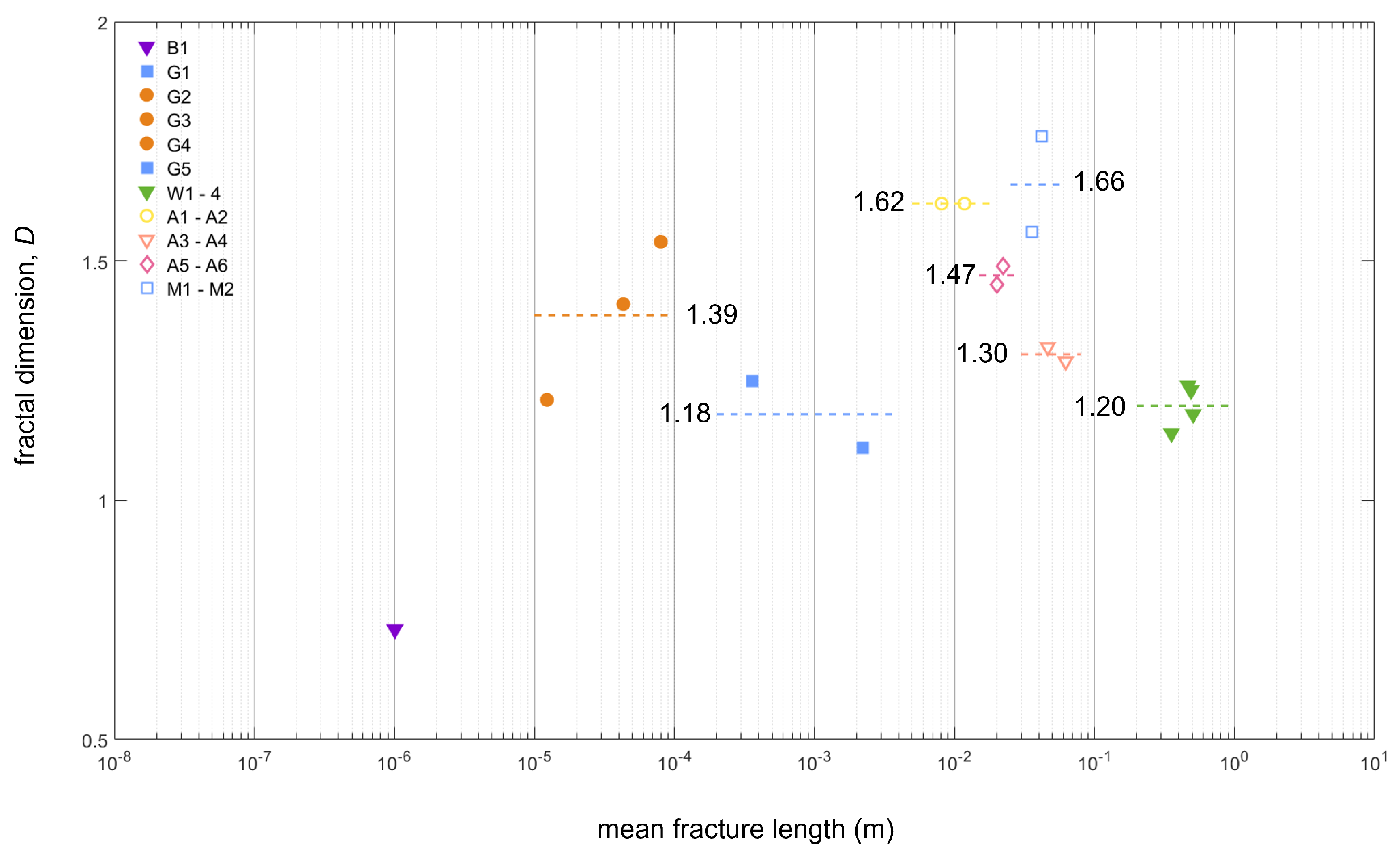
Fractal dimension was calculated for each sample listed in Table 1. Fractal dimensions for three-dimensional datasets were converted into their two-dimensional equivalent using the following relation [21,32]:
in order to compare results across the full dataset as a group. Figure 2 shows data grouped by order of magnitude and summarizes the results as follows.
Image scale: The fracture network segmented for sample B1 has a fractal dimension equal to 1.73, and therefore it is not considered fractal because D3D < 2. The average estimated fractal dimension () for a subset of the G series samples (G2, G3, and G4) was 1.39, while micro (samples G1 and G5) and macro (samples W1–W4) have close averages values of 0.18 and 0.20, respectively. This result suggests a small reduction in fracture network complexity at scales larger than 10−4 and possibly a smaller frequency of fractures as well. These observations were qualitatively made during the segmentation stage of the samples as scales increased, as well as during the reconstruction stage of the macro-scale data.
Image dimension: In order to compare fractal dimension values between 2D and 3D, we used Equation (6) to downscale the three-dimensional values of D. Acknowledging that Equation (6) is an approximation [21], a decrease in fractal dimension is observed for 3D image data as compared to 2D. This decrease coincides with an increasing length scale, as detailed above.
Fracture network origin (rock shale samples only): On average, using pyrolysis to mature kerogen and organic matter (G series) seems to produce an only slightly larger fractal dimension on the studied samples than those representing the group of natural and hydraulically fractured rocks (W series). In our dataset, micro-scale samples (G series) were subject to significant heat leading to accelerated kerogen maturation. This process tends to originate fracture clusters near and on the high organic matter concentration zones, that are arranged in laminations for these samples. Therefore, the resulting fracture networks are at least partially correlated to the sample’s total organic content (TOC). These factors were extensively discussed in [37]. As the natural/hydraulically fractured samples are only represented at macro-scale, no definitive comparison can be made in this regard, other than the slight difference denoted above.
Rock and rock analogs. The rock analog samples included in the A series are described in detail in [38,41]. As previously mentioned, the main distinction between these samples is that the rock analog material varies in fracture toughness (S) such that SA5,A6 > SA3,A4 > SA1,A2. Therefore, we subgrouped this set of samples into pairs of similar strength as described above. If we consider fractal dimension as a validation parameter for the rock analogs, the pair A5, A6 (strongest material) has the closest average fractal dimension value to the 10−5–10−4 m range (1.47 to 1.39, respectively). At the micro-scale (around 10−3 m), the A3–A4 pair (mid-strength) has the closest average to the rock shale samples of this study (1.30–1.18). The same result is obtained when the macro-scale samples (1.30 average for A3, A4 and 1.20 average for the W series) are compared. Fractal dimension is not the only validation parameter for rock analogs; however, it complements the connectivity assessment as shown in the following section. Fractal dimension helps determine whether an analog reasonably approximates some rock properties or transport behaviors.
3.2. Connectivity
In this section, the discussion revolves around the interplay between the samples’ fracture network fractal geometry and the applicability of a power-law function to their fracture length distributions. Table 2 summarizes the results of the main calculated parameters, and D, as well as the inference made on each individual fracture network’s connectivity based on inequalities (3) through (5).
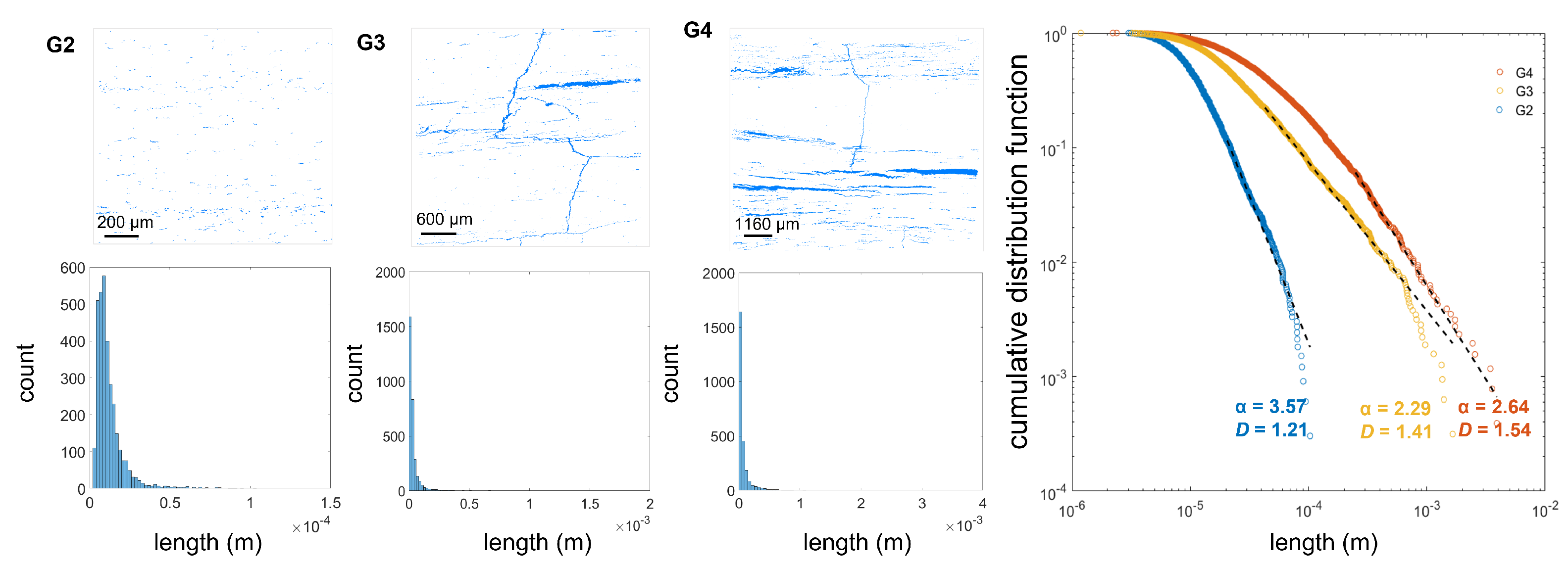
2D Shale rock images:The samples included in this group are G2, G3, and G4. The segmented fracture networks, histograms, and cumulative distribution function (cdf) curves for each sample are shown in Figure 3, along with dotted straight lines that represent the fit to power-law functions for each curve. As indicated in Table 1, the image modality is SEM for all samples. The segmented fracture network of sample G2 mostly consists of small evenly spaced fractures with an average size much smaller than the system size. As a result, sample G2 exhibits the smallest fractal dimension of the group (D = 1.21) and the largest value of (3.57). Values of > 3 suggest that connectivity is dominated by fractures of length much smaller than the system [21,24,32].
On the other hand, samples G3 (partial view) and G4 show a small number of large fractures that cut across at least half of the imaged area, along with more distinct fracture clusters with a wider range of fracture lengths, i.e., larger lacunarity, or the presence of significant fracture-free areas. The values of are larger than 2 but less than 3. This result points to the equal importance of short and large fractures for network connectivity. The fracture system of sample G3 is an example of a fracture network where the loss of connectivity caused by fractal lacunarity is compensated by the presence and connectivity provided by one or more fractures of a length close to that of the system. This balance is only achieved if < D + 1 [24]. In the case of sample G4, ≈ D + 1, suggesting that short and long fractures have equal weight on sample connectivity.
In order to interpret these results, we must consider the samples’ compositional distribution, i.e., laminations and organic matter content distribution, as well as lamination orientation. In samples G2 and G4, laminations are horizontal, and in sample G3, laminations run vertical [37]. The lamination composition of these samples alternates between large and small organic matter content. It is also important to make the distinction that the segmented section of sample G2 belongs to a small organic matter content lamination. Because the fracture networks of these samples originated from heat-induced organic matter maturation, the laminations with larger organic matter content have larger fractures and fracture clustering. This explains the short length and evenly distributed fracturing of sample G2, and the clustered, large connecting fractures found for samples G3 and G4. The interpretation of their and D values confirm these observations.
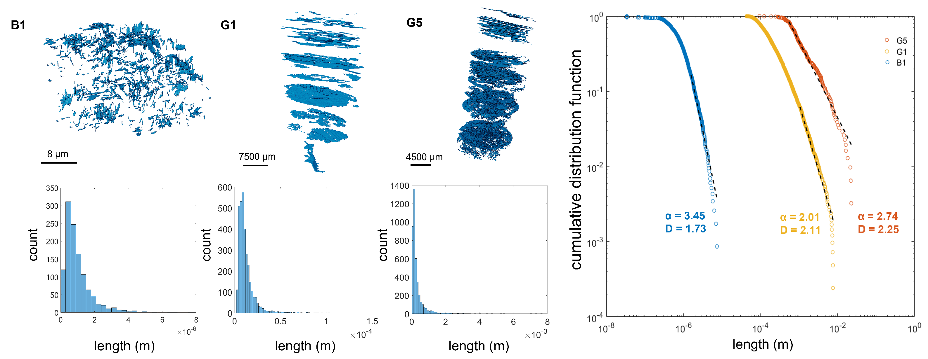
3D shale rock images—micro-scale: The samples included in this group are B1, G1, and G5. The segmented fracture networks, histograms, and cumulative distribution function (cdf) curves for each sample are shown in Figure 4, along with dotted straight lines that represent the fit to power-law functions for each curve. As indicated in Table 1, the image modality is nano-CT (also known as transmission X-ray microscope or TXM) for sample B1, and micro-CT for samples G1 and G5. The segmented fracture network of sample B1 mostly consists of small and jagged fractures of a narrow range of sizes, as its histogram shows. Similarly to sample G2, sample B1 exhibits a small fractal dimension (in fact, it is not a fractal system), and > 3; therefore, fractures much smaller than the system size are expected to control connectivity. The fracture networks of samples G1 and G5 seem to have a dual fracture system. There are a small number of large fractures that span the diameter of the sample and match the samples’ large organic matter laminations, and a large network of small fractures, mostly located on the small organic matter content laminations. Both histograms confirm the observation and their values indicate that the connectivity is dominated by both small and large fractures. Again, the fractal lacunarity of the samples is balanced out by the large fractures that span a dimension of the sample size (diameter) and the condition < D + 1 is met.
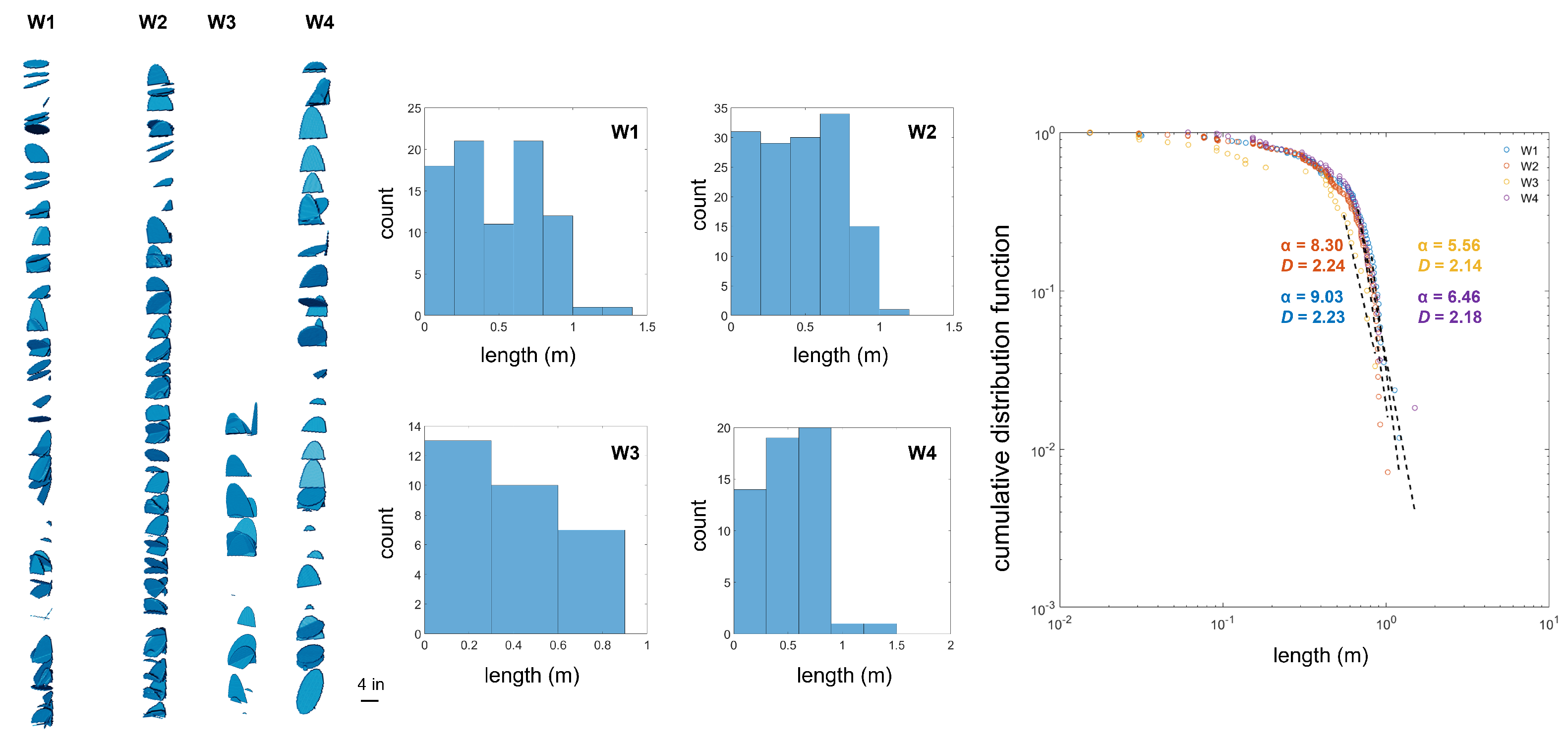
3D shale rock images—macro-scale: The samples included in this group are W1, W2, W3, and W4. The segmented fracture networks, histograms, and cumulative distribution function (cdf) curves for each sample are shown in Figure 5, along with dotted straight lines that represent the fit to power-law functions for each curve. As mentioned above, the image data for these samples do not come from direct imaging but from data reconstruction based upon the recorded fracture geometry. As a result, the reconstructions used for this study carry some uncertainty associated with any missing or inaccurate tabular data. The average fracture for this dataset consists of incline planes that start and end at the edges of the core sample. The histograms for all samples show a relative homogeneity of fracture sizes. The power-law exponent for all samples is large (≫3) and indicates that connectivity is dominated by fractures smaller than those of the system. In this case, given that > D + 1, it is expected that the fracture network connectivity increases with decreasing scale [21].
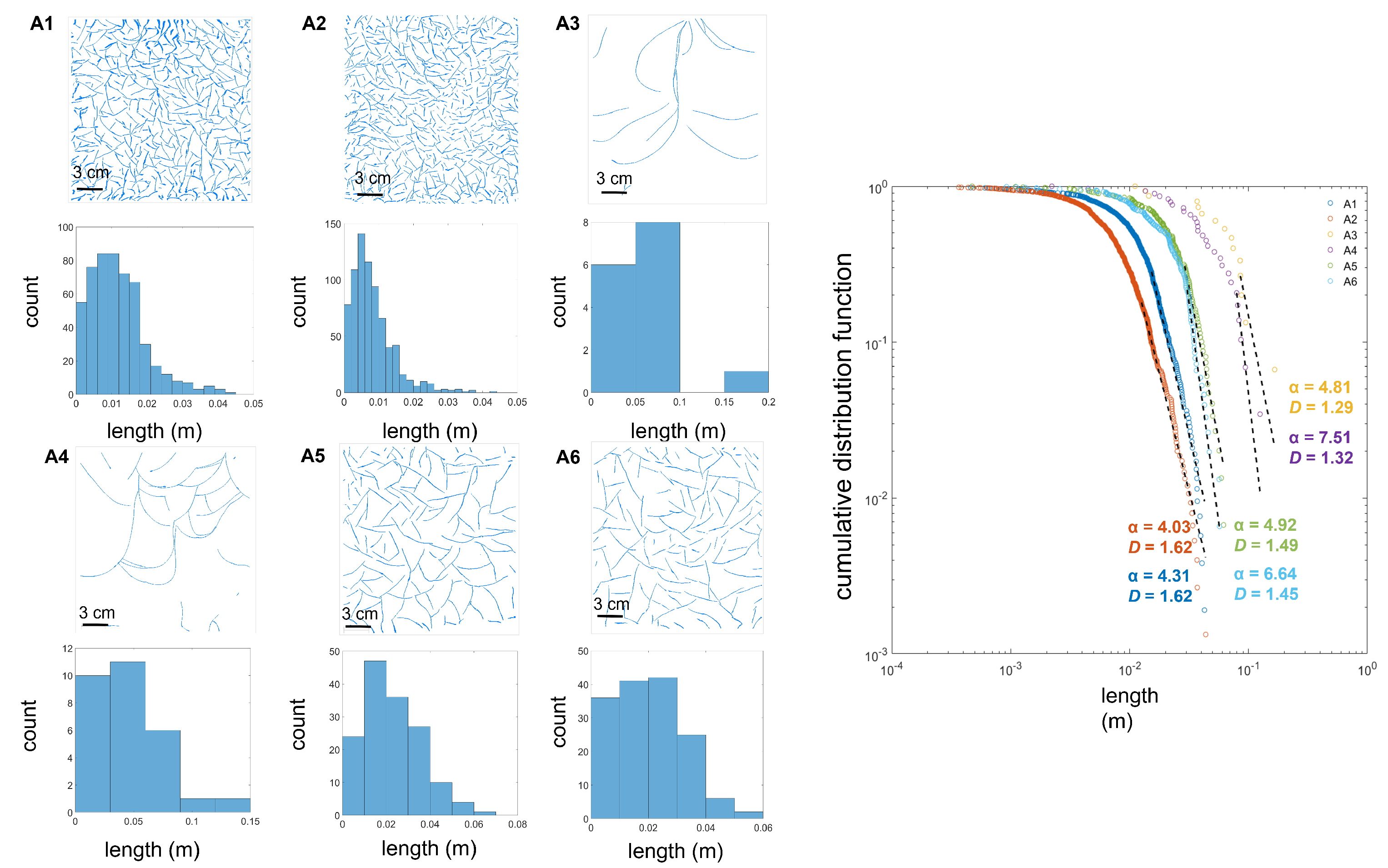
Shale rock analog images: The samples included in this group are A1–A6. The segmented fracture networks, histograms, and cumulative distribution function (cdf) curves for each sample are shown in Figure 6, along with dotted straight lines that represent the fit to power-law functions for each curve. Gelatin of increasing material strength was used as a shale rock analog, as described in [38,41]. The resulting fracture networks exhibit behaviors correlating to the gelatin tensile strength and the histograms are skewed to the left, indicating a predominance of fractures smaller than the system size. The cdf curves and their power-law fit show values of > 3, for all cases, suggesting alignment with results found for some rock shale samples. As with the macro shale rock series, > D + 1, indicating that connectivity is sustained by fracture networks of length smaller than the system.
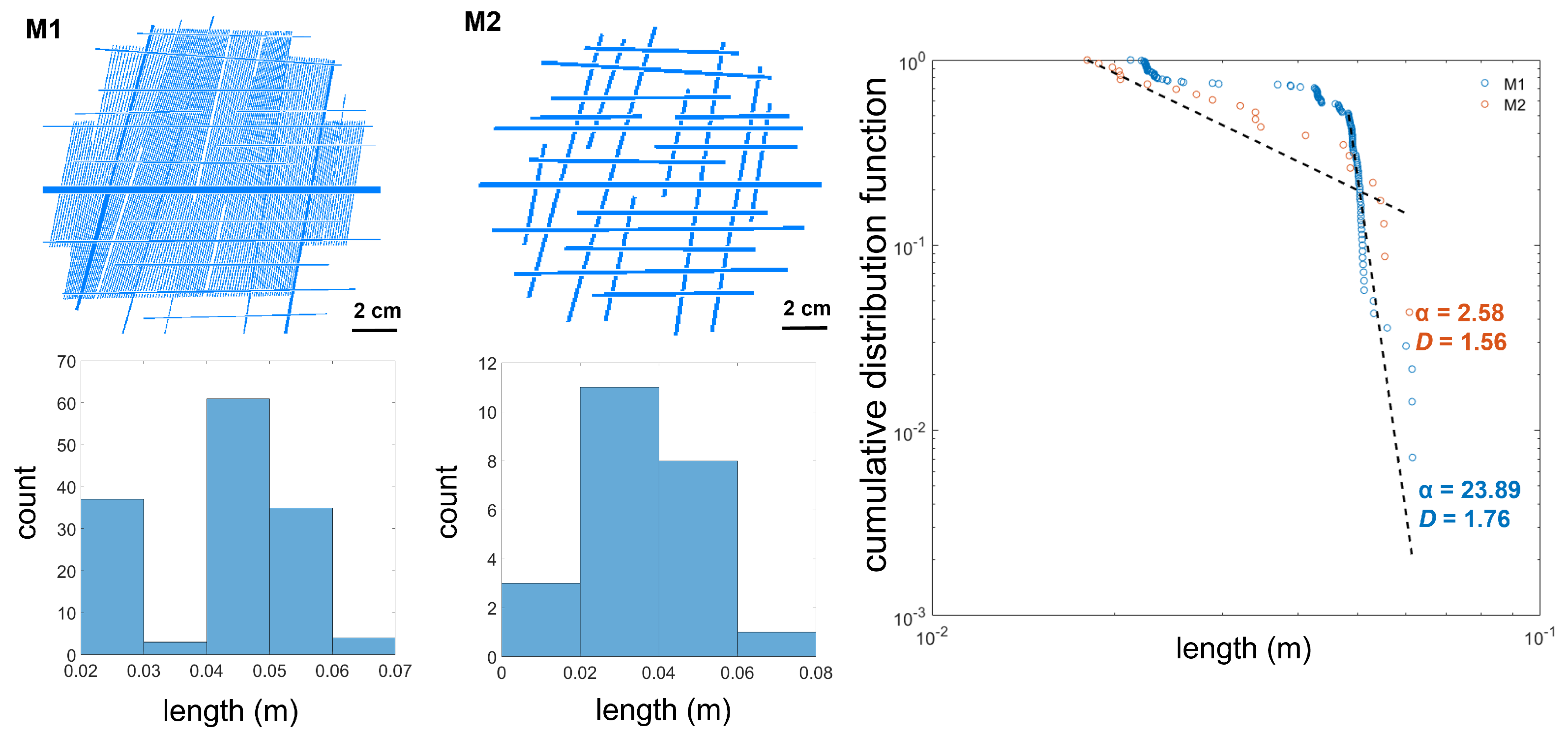
Microfluidic devices: The samples included in this group are M1 and M2. The segmented fracture networks, histograms, and cumulative distribution function (cdf) curves for each sample are shown in Figure 7, along with dotted straight lines that represent the fit to power-law functions for each curve. The design and use of these microfluidics devices was explained and detailed in [39]. The histograms show that the fracture networks of samples M1 and M2 are comprised of fractures of relative similar size. Sample M1 has a very large value, mostly for larger fracture sizes, and along with > D + 1 suggests that the smaller fractures dominate connectivity in this system. Sample M2 does not have an excellent power-law fit, but its and calculated fractal dimension suggest that connectivity will likely be dominated by both short and long fractures (2 < < 3) or be scale invariant ( ≈ D + 1).
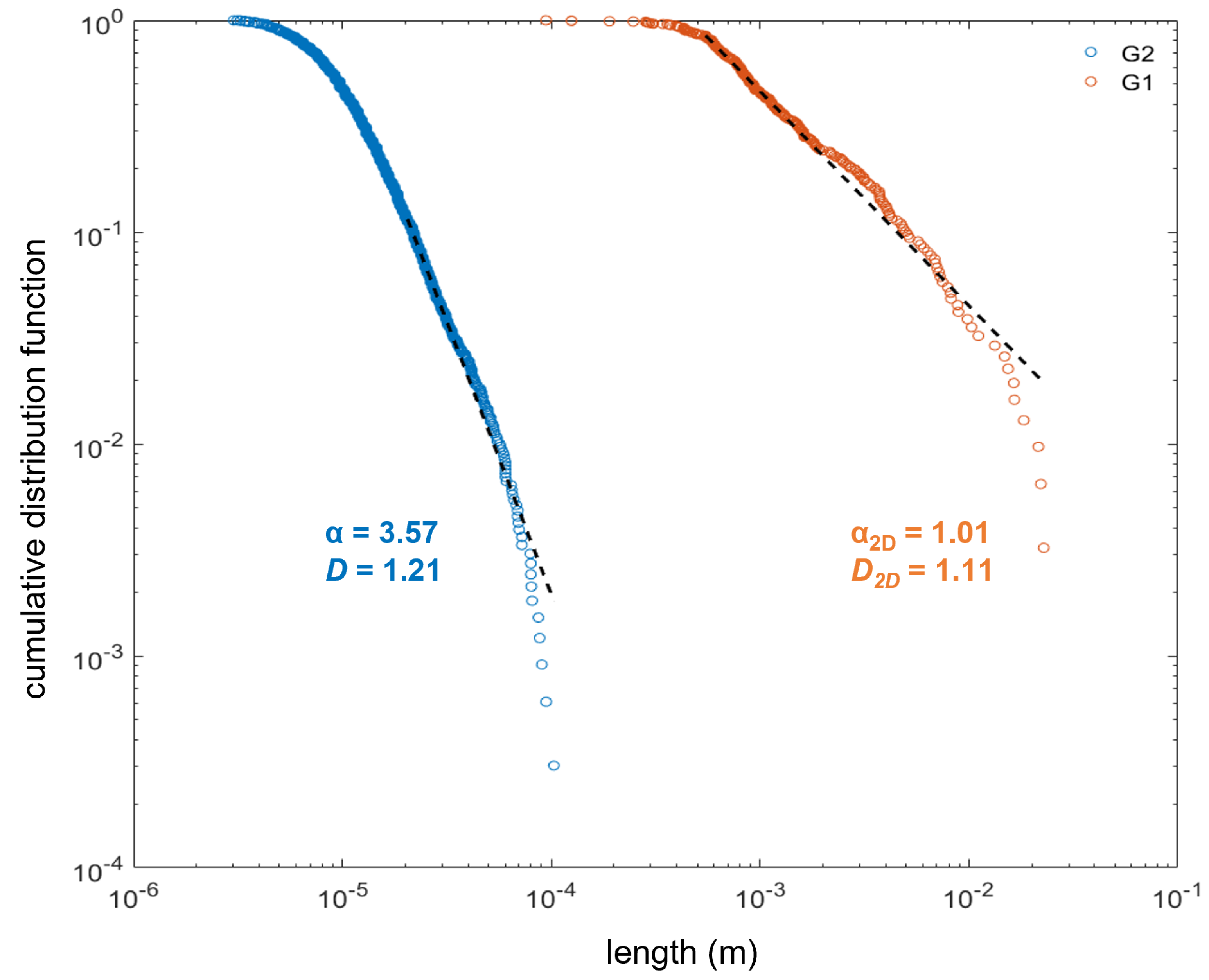
Same sample: In Table 1, datasets G1 and G2 are marked with a * to denote that they belong to the same sample, imaged at the micro- and nano-scale, respectively. Figure 8 shows the cdf curves for samples G1 and G2, along with dotted straight lines that represent the fit to power-law functions for each curve. In this case, DG2 is only slightly larger than DG1-2D equiv. (1.21 and 1.11, respectively), but their values are different (1.01 and 3.57, respectively). This difference may be partially due to connectivity distinctions between 2D and 3D networks, as well as probably due to the difference in organic content of each segmented sample area or volume, and its consequences, as previously described. Overall, it seems likely that the imaged sample area and image resolution are the main reasons the fracture length distributions diverge in this case.
Rock and rock analogs.Figure 9 shows a close up of cdf curves for the shale rock samples G2 and G5 shown in Figure 4 in addition to the curves representing the rock analog samples A1–A6 and M1 and M2 microfluidic devices, from Figure 6 and Figure 7, respectively. The curves were normalized by sample surface area. Solid and dotted trend lines were superimposed on some of these curves to characterize the connectivity and continuity between samples. In particular, the fracture network on sample G1 seems to correlate with the rock analogs A5 and A6 with the dotted trend line of = 1.4; whilst sample G5 follows a connecting trend line to rock analogs A1 and A2, with the solid trend line of = 1.8. These results validate gelatin as a rock analog for thermally induced fracture networks, consistent with the original premise [38,41].
The distribution curves for the microfluidic devices do not seem to match the shale rock curves by one or two orders of magnitude. An increase in the fractured area, while preserving the current fracture network lengths and designs, may be all the adjustment needed to shift these curves closer to the path of the shale rock curves, and thus enhance their modeling potential.
3.3. Multiscale Length Distribution
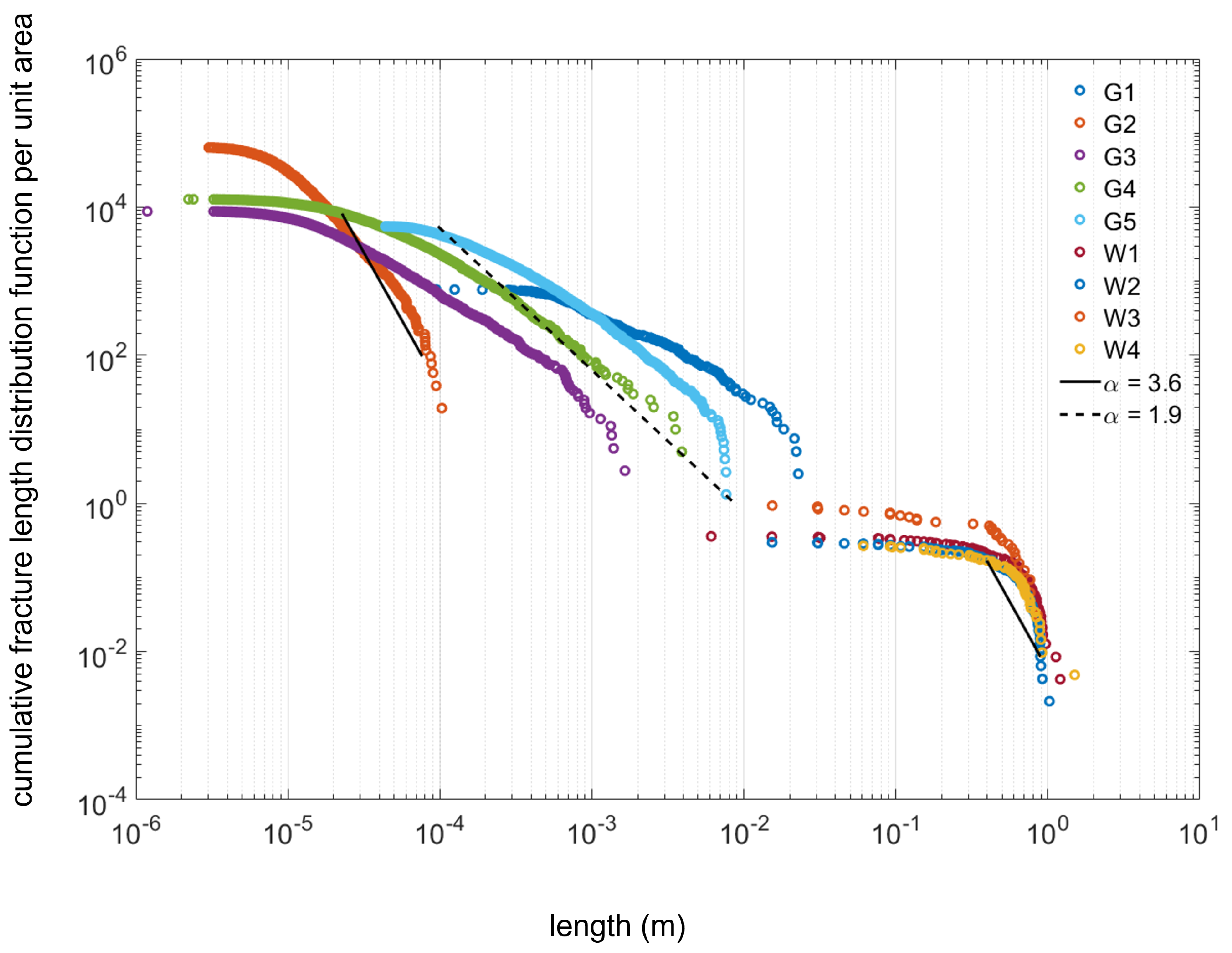
Shale rock only: Cumulative fracture length distribution curves are plotted in Figure 10 for all the shale rock fractal samples included in this study (the curve for sample B1 is therefore not shown). Curve values were normalized by sample surface area, and trend lines were traced in order to find the connectivity regime continuity throughout the scales [24,36] should they exist. The fractal fracture network scale range covered in this study spans the 10−6–100 m interval. There is a lack of data for the length range between 10−2 and 10−1 m, that makes that scale range underrepresented. A data source for this scale could possibly be addressed with medical CT scanner images.
Two trend lines were traced over the curve groups. A solid line is shown over the curve for sample G2, and over the curves for samples W1–W4. The power-law exponent for this trend line is = 3.6. A dotted trend line is shown over the curve group of samples G1, G3, G4, and G5, with a smaller slope equivalent to = 1.6. We found that a single trend line would not be able to encompass the curves for all samples, and that samples could in fact be grouped by the fracture network origin, as denoted in Table 1. An exception to this grouping criterion is sample G1, that was exposed to heat-induced or artificial thermal maturation, but is not grouped with the other similar samples. Because this sample does not exhibit the same organic matter distribution as the other samples, it could be technically considered not part of the HI group. The cdf curve for sample G1 supports this claim, and the = 3.6 trend line is a better fit than the = 1.9 line.
These results suggest that the fracture networks within unconventional rocks are created in an important and distinctive factor with respect to their fracture network connectivity and scaling. For the natural or hydraulically fractured dataset group (samples G2 and W1 through W4), the power-law exponent is always >3, indicating that connectivity is controlled by fractures much smaller than the system size. Furthermore, > D + 1 suggests that the connectivity decreases with scale. On the other hand, the heat-induced organic matter maturation group (samples G1 and G3–G5), have values such that 2 < < 3, suggesting that both small and large fractures contribute to connectivity, although < D + 1 points towards the dominance large fractures. The segmented images for these samples in Figure 3 and Figure 4 support these calculations, showing several fractures—of the same size as those of the system—that seem to run across the sample areas, connecting distant fracture clusters. These large fracture areas coincide with large organic matter content laminations.
4. Conclusions
Fractal dimension and the statistics of fracture length are geometrical information widely regarded as characteristic of most natural and induced fracture patterns. Knowledge of these key characteristics aids efforts to construct digital representations of fractured systems. In this study, we characterized a number of fracture networks imaged within shale rock samples and shale rock analogs by analyzing fractal dimensions and fitting fracture length distributions to power-law functions. We applied them as tools to characterize fracture networks originating from different processes: maturation due to the pyrolysis of organic matter components as well as natural and hydraulically induced fractures. The specific connectivity criteria applied here are explained at length in [21,24,32]. Specifically, we conclude the following:
- Throughout a sample size range spanning from 10−6 to 100 m, most sample systems show a power-law exponent > 3, suggesting that fractures one or more orders of magnitude smaller than the system size control connectivity and classic rules of percolation theory apply. These fractal fracture network samples also fall in the > D + 1 category, indicating that connectivity decreases with system scale. These samples belong to the natural/hydraulically fractured group.
- Fractures in the samples matured using pyrolysis (G1, G3, G4, and G5) correlate with a different connectivity regime than the natural/hydraulic fractures. These fractures fit power-law exponents such that 2 < < 3, suggesting that a combination of small and large fractures interact to determine connectivity, but they also conform to < D + 1, such that larger fractures prevail in system connectivity. This effect increases with system scale. Given the fracture length distribution shown on their histograms and their segmented images, it is probable that the larger fractures (of the same order of magnitude as system length) are more dominant than smaller fractures (one or more orders of magnitude smaller than the system).
- The distribution and abundance of organic matter of the shale samples has a direct and predominant effect on the distribution and clustering of the resulting fracture networks if the rock is (naturally or artificially) matured. In the samples included in this study, this effect resulted in large fractures located within the laminations of samples with a large amount of organic matter. These fractures dominate connectivity. In the case of hydraulic fracturing, the process is correlated to the mechanical features of the rock and the fracturing parameters that overall produces fracture networks with connectivity most likely dominated by smaller system size fractures.
- Gelatin is found to be an accurate rock analog for maturation-induced fractures as validated through multiscale connectivity trends.
Author Contributions
Conceptualization, methodology, software, validation, B.V.; formal analysis, B.V. and A.R.K.; investigation, data curation, writing—original draft preparation, B.V.; resources, writing—review and editing, supervision, project administration, funding acquisition, A.R.K. All authors have read and agreed to the published version of the manuscript.
Funding
This research was funded by the Center for Mechanistic Control of Unconventional Formations (CMC-UF), an Energy Frontier Research Center funded by the U.S. Department of Energy, Office of Science under DOE (BES) Award DE-SC0019165.
Institutional Review Board Statement
Not applicable.
Informed Consent Statement
Not applicable.
Data Availability Statement
Fracture network images are available on the Digital Rocks Portal: https://doi.org/10.17612/15RS-9J28.
Acknowledgments
Parts of this research were carried out at the Stanford Synchrotron Radiation Lightsource, at the Directorate of SLAC National Accelerator Laboratory, and at an Office of Science User Facility operated by the US Department of Energy Office of Science by Stanford University. The authors thank C.M. Ross, T. Kim, and B. Ling et al. for allowing the use of their data in this study.
Conflicts of Interest
The authors declare no conflict of interest.
Abbreviations
The following abbreviations are used in this manuscript:
| power-law function exponent | |
| D | fractal dimension |
| cdf | cumulative distribution function |
| HI | heat-induced organic matter maturation |
| N, HF | natural and hydraulically fractured rock samples |
References
- Gale, J.F.W.; Holder, J. Natural fractures in some US shales and their importance for gas production. In Petroleum Geology: From Mature Basins to New Frontiers, Proceedings of the 7th Petroleum Geology Conference; Geological Society of London: London, UK, 2010. [Google Scholar] [CrossRef]
- Allix, P.; Burnham, A.; Fowler, T.; Herron, M.; Kleinberg, R.; Symington, B. Coaxing oil from shale. Oilfield Rev. 2010, 22, 4–15. [Google Scholar]
- Akkutlu, I.Y.; Fathi, E. Multiscale gas transport in shales with local kerogen heterogeneities. SPE J. 2012, 17, 1002–1011. [Google Scholar] [CrossRef] [Green Version]
- Aljamaan, H.; Alnoaimi, K.; Kovscek, A. In-depth experimental investigation of shale physical and transport properties. In Proceedings of the Unconventional Resources Technology Conference, Denver, CO, USA, 12–14 August 2013; pp. 1120–1129. [Google Scholar]
- Aljamaan, H.; Ross, C.M.; Kovscek, A.R. Multiscale Imaging of Gas Storage in Shales. SPE J. 2017, 22, 1760–1777. [Google Scholar] [CrossRef]
- Alnoaimi, K.R.; Duchateau, C.; Kovscek, A. Characterization and measurement of multi-scale gas transport in shale core samples. In Proceedings of the Unconventional Resources Technology Conference, Denver, CO, USA, 25–27 August 2014; pp. 1140–1158. [Google Scholar]
- Vega, B.; Andrews, J.C.; Liu, Y.; Gelb, J.; Kovscek, A. Nanoscale visualization of gas shale pore and textural features. In Proceedings of the Unconventional Resources Technology Conference, Denver, CO, USA, 12–14 August 2013; pp. 1603–1613. [Google Scholar]
- Sondergeld, C.H.; Ambrose, R.J.; Rai, C.S.; Moncrieff, J. Micro-structural studies of gas shales. In Proceedings of the SPE Unconventional Gas Conference, Pittsburgh, PA, USA, 23–25 February 2010. [Google Scholar]
- Elgmati, M.M.; Zhang, H.; Bai, B.; Flori, R.E.; Qu, Q. Submicron-pore characterization of shale gas plays. In Proceedings of the North American Unconventional Gas Conference and Exhibition, The Woodlands, TX, USA, 14–16 June 2011. [Google Scholar]
- Curtis, M.E.; Ambrose, R.J.; Sondergeld, C.H. Structural characterization of gas shales on the micro-and nano-scales. In Proceedings of the Canadian Unconventional Resources and International Petroleum Conference, Calgary, AB, Canada, 19–21 October 2010. [Google Scholar]
- Energy Technology Perspectives. IEA Energy Technology Perspectives 2008–Scenarios and Strategies to 2050; International Energy Agency: Paris, France, 2008. [Google Scholar]
- Nuttall, B.C.; Drahovzal, J.A.; Eble, C.; Bustin, R.M. CO2 sequestration in gas shales of Kentucky. In Proceedings of the Oral Presentation at AAPG Annual Convention, Calgary, AB, Canada, 19–22 June 2005; pp. 19–22. [Google Scholar]
- Khosrokhavar, R.; Griffiths, S.; Wolf, K.H. Shale Gas Formations and Their Potential for Carbon Storage: Opportunities and Outlook. Environ. Process. 2014, 1, 595–611. [Google Scholar] [CrossRef] [Green Version]
- Tao, Z.; Clarens, A. Estimating the Carbon Sequestration Capacity of Shale Formations Using Methane Production Rates. Environ. Sci. Technol. 2013, 47, 11318–11325. [Google Scholar] [CrossRef] [PubMed]
- Mohagheghian, E.; Hassanzadeh, H.; Chen, Z. CO2 sequestration coupled with enhanced gas recovery in shale gas reservoirs. J. CO2 Util. 2019, 34, 646–655. [Google Scholar] [CrossRef]
- Godec, M.; Koperna, G.; Petrusak, R.; Oudinot, A. Potential for enhanced gas recovery and CO2 storage in the Marcellus Shale in the Eastern United States. Int. J. Coal Geol. 2013, 118, 95–104. [Google Scholar] [CrossRef]
- Lord, A.S.; Kobos, P.H.; Borns, D.J. Geologic storage of hydrogen: Scaling up to meet city transportation demands. Int. J. Hydrog. Energy 2014, 39, 15570–15582. [Google Scholar] [CrossRef] [Green Version]
- Tarkowski, R.; Uliasz-Misiak, B.; Tarkowski, P. Storage of hydrogen, natural gas, and carbon dioxide – Geological and legal conditions. Int. J. Hydrog. Energy 2021, 46, 20010–20022. [Google Scholar] [CrossRef]
- Gale, J.; Laubach, S.; Olson, J.; Eichhubl, P.; Fall, A. Natural fractures in shale: A review and new observations. AAPG Bull. 2014, 98, 2165–2216. [Google Scholar] [CrossRef]
- Gale, J.F.W.; Elliott, S.J.; Laubach, S.E. Hydraulic Fractures in Core From Stimulated Reservoirs: Core Fracture Description of HFTS Slant Core, Midland Basin, West Texas. In Proceedings of the SPE/AAPG/SEG Unconventional Resources Technology Conference, Houston, TX, USA, 23–25 July 2018. [Google Scholar] [CrossRef]
- Darcel, C.; Bour, O.; Davy, P.; de Dreuzy, J.R. Connectivity properties of two-dimensional fracture networks with stochastic fractal correlation. Water Resour. Res. 2003, 39. [Google Scholar] [CrossRef]
- Gasparrini, M.; Sassi, W.; Gale, J.F. Natural sealed fractures in mudrocks: A case study tied to burial history from the Barnett Shale, Fort Worth Basin, Texas, USA. Mar. Pet. Geol. 2014, 55, 122–141. [Google Scholar] [CrossRef] [Green Version]
- Gale, J.; Reed, R.; Holder, J. Natural fractures in the Barnett Shale and their importance for hydraulic fracture treatments. AAPG Bull. 2007, 91, 603–622. [Google Scholar] [CrossRef]
- Davy, P.; Bour, O.; Dreuzy, J.R.D.; Darcel, C. Flow in multiscale fractal fracture networks. In Fractal Analysis for Natural Hazards; Geological Society of London: London, UK, 2006. [Google Scholar] [CrossRef]
- Mandelbrot, B. How Long Is the Coast of Britain? Statistical Self-Similarity and Fractional Dimension. Science 1967, 156, 636–638. [Google Scholar] [CrossRef] [PubMed] [Green Version]
- Mandelbrot, B. Form, chance and dimension. In Chance and Dimension; Freeman: San Francisco, CA, USA, 1977; pp. 1–234. [Google Scholar]
- Barton, C.; Zoback, M. Self-similar distribution and properties of macroscopic fractures at depth in crystalline rock in the Cajon Pass Scientific Drill Hole. J. Geophys. Res. Solid Earth 1992, 97, 5181–5200. [Google Scholar] [CrossRef]
- Watanabe, K.; Takahashi, H. Fractal geometry characterization of geothermal reservoir fracture networks. J. Geophys. Res. Solid Earth 1995, 100, 521–528. [Google Scholar] [CrossRef]
- Xia, Y.; Cai, J.; Wei, W.; Hu, X.; Wang, X.; Ge, X. A new method for calculating fractal dimensions of porous media based on pore size distribution. Fractals 2018, 26, 1850006. [Google Scholar] [CrossRef]
- Velde, B.; Dubois, J.; Moore, D.; Touchard, G. Fractal patterns of fractures in granites. Earth Planet. Sci. Lett. 1991, 104, 25–35. [Google Scholar] [CrossRef]
- Miao, T.; Yang, S.; Long, Z.; Yu, B. Fractal analysis of permeability of dual-porosity media embedded with random fractures. Int. J. Heat Mass Transf. 2015, 88, 814–821. [Google Scholar] [CrossRef]
- Bonnet, E.; Bour, O.; Odling, N.; Davy, P.; Main, I.; Cowie, P.; Berkowitz, B. Scaling of fracture systems in geological media. Rev. Geophys. 2001, 39, 347–383. [Google Scholar] [CrossRef] [Green Version]
- Hazra, B.; Wood, D.; Kumar, S.; Saha, S.; Dutta, S.; Kumari, P.; Singh, A. Fractal disposition, porosity characterization and relationships to thermal maturity for the Lower Permian Raniganj basin shales, India. J. Nat. Gas Sci. Eng. 2018, 59, 452–465. [Google Scholar] [CrossRef]
- Chelidze, T.; Gueguen, Y. Evidence of fractal fracture. Int. J. Rock Mech. Min. Sci. Geomech. Abstr. 1990, 27, 223–225. [Google Scholar] [CrossRef]
- Vignes-Adler, M.; Page, A.L.; Adler, P. Fractal analysis of fracturing in two African regions, from satellite imagery to ground scale. Tectonophysics 1991, 196, 69–86. [Google Scholar] [CrossRef]
- Chabani, A.; Trullenque, G.; Ledésert, B.A.; Klee, J. Multiscale Characterization of Fracture Patterns: A Case Study of the Noble Hills Range (Death Valley, CA, USA), Application to Geothermal Reservoirs. Geosciences 2021, 11, 280. [Google Scholar] [CrossRef]
- Kim, T.; Ross, C.; Guan, K.; Burnham, A.; Kovscek, A. Permeability and Porosity Evolution of Organic-Rich Shales from the Green River Formation as a Result of Maturation. SPE J. 2020, 25, 1377–1405. [Google Scholar] [CrossRef]
- Vega, B.; Yang, J.; Tchelepi, H.; Kovscek, A. Investigation of Stress Field and Fracture Development During Shale Maturation Using Analog Rock Systems. Transp. Porous Media 2019, 131, 503–535. [Google Scholar] [CrossRef]
- Ling, B.; Khan, H.J.; Druhan, J.L.; Battiato, I. Multi-Scale Microfluidics for Transport in Shale Fabric. Energies 2021, 14, 21. [Google Scholar] [CrossRef]
- Vega, B.; Ross, C.M.; Kovscek, A.R. Imaging-Based Characterization of Calcite-Filled Fractures and Porosity in Shales. SPE J. 2015, 20, 810–823. [Google Scholar] [CrossRef]
- Vega, B.; Kovscek, A. A systematic study of internal gas generation in shale source rocks using analog experiments. J. Pet. Sci. Eng. 2019, 173, 209–221. [Google Scholar] [CrossRef]
- Clauset, A.; Shalizi, C.R.; Newman, M.E.J. Power-Law Distributions in Empirical Data. SIAM Rev. 2009, 51, 661–703. [Google Scholar] [CrossRef] [Green Version]
Figure 1.
Multimodal, multiscale image dataset. The labels on the images correspond to those listed in Table 1.
Figure 1.
Multimodal, multiscale image dataset. The labels on the images correspond to those listed in Table 1.

Figure 2.
Fractal dimensions calculated for the image dataset.

Figure 3.
Segmented fracture networks, histograms, and cumulative distribution function for 2D shale rock images corresponding to samples G2, G3, and G4.
Figure 3.
Segmented fracture networks, histograms, and cumulative distribution function for 2D shale rock images corresponding to samples G2, G3, and G4.

Figure 4.
Segmented fracture networks and cumulative distribution function for 3D shale rock images corresponding to samples B1, G1, and G5.
Figure 4.
Segmented fracture networks and cumulative distribution function for 3D shale rock images corresponding to samples B1, G1, and G5.

Figure 5.
Segmented fracture networks and cumulative distribution function for 3D shale rock images corresponding to samples W1, W2, W3, and W4.
Figure 5.
Segmented fracture networks and cumulative distribution function for 3D shale rock images corresponding to samples W1, W2, W3, and W4.

Figure 6.
Segmented fracture networks and cumulative distribution function for shale rock analog images corresponding to samples A1, A2, A3, A4, A5, and A6.
Figure 6.
Segmented fracture networks and cumulative distribution function for shale rock analog images corresponding to samples A1, A2, A3, A4, A5, and A6.

Figure 7.
Segmented fracture networks and cumulative distribution function for shale rock microfluidic device images corresponding to samples M1 and M2.
Figure 7.
Segmented fracture networks and cumulative distribution function for shale rock microfluidic device images corresponding to samples M1 and M2.

Figure 8.
Fracture length distribution for rock shale samples G1 and G2.

Figure 9.
Fracture length distribution for shale samples G2 and G5; rock analog samples A1, A2, A3, A4, A5, and A6; and microfluidic models M1 and M2.
Figure 9.
Fracture length distribution for shale samples G2 and G5; rock analog samples A1, A2, A3, A4, A5, and A6; and microfluidic models M1 and M2.

Figure 10.
Multiscale fracture length distribution for the full set of rock image data.


Table 1.
Image data details.
| Sample | Sample Size Length Units | Image Resolution | Euclidean Dimension | Image Modality | Fracture Origin | Data Provenance |
|---|---|---|---|---|---|---|
| B1 | m | 31.2 nm/vx | 3 | nano-CT | N | [40] |
| G1 * | cm | 30.58 m/vx | 3 | micro-CT | HI | [37] |
| G2 * | mm | 540 nm/px | 2 | SEM | HI | [37] |
| G3 | mm | 540 nm/px | 2 | SEM | HI | [37] |
| G4 | mm | 540 nm/px | 2 | SEM | HI | [37] |
| G5 | mm | 5.11 m/vx | 3 | micro-CT | HI | [37] |
| W1 | m | 0.3 × 0.3 × 2.4 mm/vx | 3 | tabular data | N, F | unpublished |
| W2 | m | 0.3 × 0.3 × 2.4 mm/vx | 3 | tabular data | N, F | unpublished |
| W3 | m | 0.3 × 0.3 × 2.4 mm/vx | 3 | tabular data | N, F | unpublished |
| W4 | m | 0.3 × 0.3 × 2.4 mm/vx | 3 | tabular data | N, F | unpublished |
| A1 | cm | 60.8 m/px | 2 | DSLR camera | N/A | [38] |
| A2 | cm | 60.8 m/px | 2 | DSLR camera | N/A | [38] |
| A3 | cm | 60.8 m/px | 2 | DSLR camera | N/A | [38] |
| A4 | cm | 60.8 m/px | 2 | DSLR camera | N/A | [38] |
| A5 | cm | 60.8 m/px | 2 | DSLR camera | N/A | [38] |
| A6 | cm | 60.8 m/px | 2 | DSLR camera | N/A | [38] |
| M1 | mm | 244.7 m/px | 2 | graphics | N/A | [39] |
| M2 | mm | 117.1 m/px | 2 | graphics | N/A | [39] |
* images from the same sample.
Table 2.
Connectivity results.
| Sample | Alpha () | D | Connectivity Dominance |
|---|---|---|---|
| B1 | 3.45 | 1.73 | small fractures |
| G1 | 2.01 | 2.11 | transitional towards large fractures |
| G2 | 3.57 | 1.21 | small fractures |
| G3 | 2.29 | 1.41 | transitional toward large fractures |
| G4 | 2.64 | 1.54 | self-similar, invariant |
| G5 | 2.74 | 2.25 | transitional toward large fractures |
| W1 | 9.03 | 2.23 | small fractures |
| W2 | 8.30 | 2.24 | small fractures |
| W3 | 5.56 | 2.14 | small fractures |
| W4 | 6.46 | 2.18 | small fractures |
| A1 | 4.31 | 1.62 | small fractures |
| A2 | 4.03 | 1.62 | small fractures |
| A3 | 4.81 | 1.29 | small fractures |
| A4 | 7.51 | 1.32 | small fractures |
| A5 | 4.92 | 1.49 | small fractures |
| A6 | 6.64 | 1.45 | small fractures |
| M1 | 23.89 | 1.76 | small fractures |
| M2 | 2.58 | 1.56 | self-similar, invariant |
Publisher’s Note: MDPI stays neutral with regard to jurisdictional claims in published maps and institutional affiliations. |
© 2022 by the authors. Licensee MDPI, Basel, Switzerland. This article is an open access article distributed under the terms and conditions of the Creative Commons Attribution (CC BY) license (https://creativecommons.org/licenses/by/4.0/).
Share and Cite
MDPI and ACS Style
Vega, B.; Kovscek, A.R. Fractal Characterization of Multimodal, Multiscale Images of Shale Rock Fracture Networks. Energies 2022, 15, 1012. https://doi.org/10.3390/en15031012
AMA Style
Vega B, Kovscek AR. Fractal Characterization of Multimodal, Multiscale Images of Shale Rock Fracture Networks. Energies. 2022; 15(3):1012. https://doi.org/10.3390/en15031012
Chicago/Turabian StyleVega, Bolivia, and Anthony R. Kovscek. 2022. "Fractal Characterization of Multimodal, Multiscale Images of Shale Rock Fracture Networks" Energies 15, no. 3: 1012. https://doi.org/10.3390/en15031012
Note that from the first issue of 2016, this journal uses article numbers instead of page numbers. See further details here.