
Stratigraphically Controlled Stress Variations at the Hydraulic Fracture Test Site-1 in the Midland Basin, TX

Department of Geophysics, School of Earth Sciences, Stanford University, Stanford, CA 94305, USA
*
Author to whom correspondence should be addressed.
Energies 2021, 14(24), 8328; https://doi.org/10.3390/en14248328
Submission received: 26 October 2021
/
Revised: 24 November 2021
/
Accepted: 29 November 2021
/
Published: 10 December 2021
(This article belongs to the Special Issue Development of Unconventional Reservoirs 2021)
Abstract
:We investigated the relationship between stratigraphy, stress, and microseismicity at the Hydraulic Fracture Test Site-1. The site comprises two sets of horizontal wells in the Wolfcamp shale and a deviated well drilled after hydraulic fracturing. Regional stresses indicate normal/strike-slip faulting with E-W compression. Stress measurements in vertical and horizontal wells show that the minimum principal stress varies with depth. Strata with high clay and organic content show high values of the least compressive stress, consistent with the theory of viscous stress relaxation. By integrating data from core, logs, and the hydraulic fracturing stages, we constructed a stress profile for the Wolfcamp sequence, which predicts how much pressure is required for hydraulic fracture growth. We applied the results to fracture orientation data from image logs to determine the population of pre-existing faults that are expected to slip during stimulation. We also determined microseismic focal plane mechanisms and found slip on steeply dipping planes striking NW, consistent with the orientations of potentially active faults predicted by the stress model. This case study represents a general approach for integrating stress measurements and rock properties to predict hydraulic fracture growth and the characteristics of injection-induced microseismicity.
1. Introduction
Horizontal drilling and multi-stage hydraulic fracturing are needed to stimulate production from unconventional petroleum reservoirs due to their extremely low permeability. Hydraulic fractures create new surface area and deliver fluid pressure to pre-existing fractures, causing them to slip and increase the area of contact where hydrocarbons can diffuse out the low permeability matrix. Efficient production and safe stimulation depends on the ability to control the growth of hydraulic fractures and limit fluid injection to target intervals. Hydraulic fractures are able to propagate when fluid pressure exceeds the least compressive stress. Thus, the least compressive stress determines the fluid pressure needed for hydraulic fracture growth from layer to layer as well as the orientations of pre-existing faults that may slip during fluid injection.
In this study, we investigated the impacts of stratigraphically controlled variations of the least compressive stress on hydraulic fracturing by applying the of viscous stress relaxation to a dataset from the Hydraulic Fracturing Test Site-1 (HFTS-1). In a series of papers, Sone and Zoback (2013b, 2014a,b) used laboratory deformation experiments and field data to show that the differential stress supported by a particular lithology (the difference between the maximum and minimum principal stresses) is determined by its capacity to undergo viscoplastic stress relaxation over time [1,2,3]. In a normal/strike-slip faulting environment, stress relaxation signifies that the magnitude of minimum horizontal stress, Shmin, increases with respect to the maximum principal stress [4]. In context of layered sequences, this implies that lithofacies that undergo more stress relaxation could act as barriers to vertical hydraulic fracture growth. Sone and Zoback (2013b) found that within the same basin, rocks with more clay minerals and total organic carbon (TOC), the most compliant components of the matrix, are expected to undergo greater stress relaxation. Sone and Zoback (2014b) used laboratory data to model viscous stress relaxation in the Barnett shale and successfully predicted where drilling induced tensile fractures would form [3]. Singh (2021) applied the model to another unconventional dataset and found that the model predictions were consistent with measurements of Shmin from diagnostic formation integrity tests (DFITs) [5]. This underscores the importance of accounting for how variations in viscous deformation properties impact stress magnitudes as a function of depth.
Several recent studies have applied the theory of viscous stress relaxation to characterize stress variations and their impact on hydraulic fracture growth. Singh et al. (2020) investigated the effect of stress layering on hydraulic fracture growth through numerical modeling [6]. Their models demonstrate that the minimum horizontal stress Shmin is the primary control on where hydraulic fractures propagate and also impacts operational design, specifically stage length and perforation cluster spacing. Ma and Zoback (2020) applied the viscous stress relaxation model to calculate variations of the minimum horizontal stress along the length of horizontal wells in the Woodford shale that are drilled across different lithofacies [7]. They observed variations in the instantaneous shut-in pressure (ISIP) of hydraulic fracturing stages that were correlated with changing lithology. However, since ISIPs are not the most reliable indicator of Shmin, Ma and Zoback (2020) estimated the variations in Shmin by calculating stress relaxation based on empirical correlations of elastic stiffness and viscoelastic compliance from laboratory data. McCormick et al. (2021) applied the Ma and Zoback (2020) correlation to a VTI elasticity model and predicted Shmin as a function of depth in the Niobrara shale [8]. They also studied the distribution of induced microseismic events as an indicator of where leak-off from hydraulic fractures occurred and found that layers with high values of Shmin acted as barriers to vertical hydraulic fracture growth. In addition, they found the that the onset of microseismicity was delayed during hydraulic stimulation of high stress layers, likely due to the longer time needed for fluid pressure to induce slip.
While previous studies have successfully characterized and modeled stress variations in unconventional reservoirs, their ability to interpret the relationship between stress and stratigraphy is often limited by the lack of reliable stress measurements. If laboratory measurements of rock deformation properties are not available for calculating stress relaxation, wellbore stress measurements are essential to understand how variations in stratigraphy and rock properties give rise to variations in stress. Here, we develop a framework for predicting patterns of hydraulic fracture growth and microseismicity based on stratigraphic stress variations using the publicly available HFTS-1 dataset.
2. Hydraulic Fracture Test Site-1
2.1. Regional Stress State
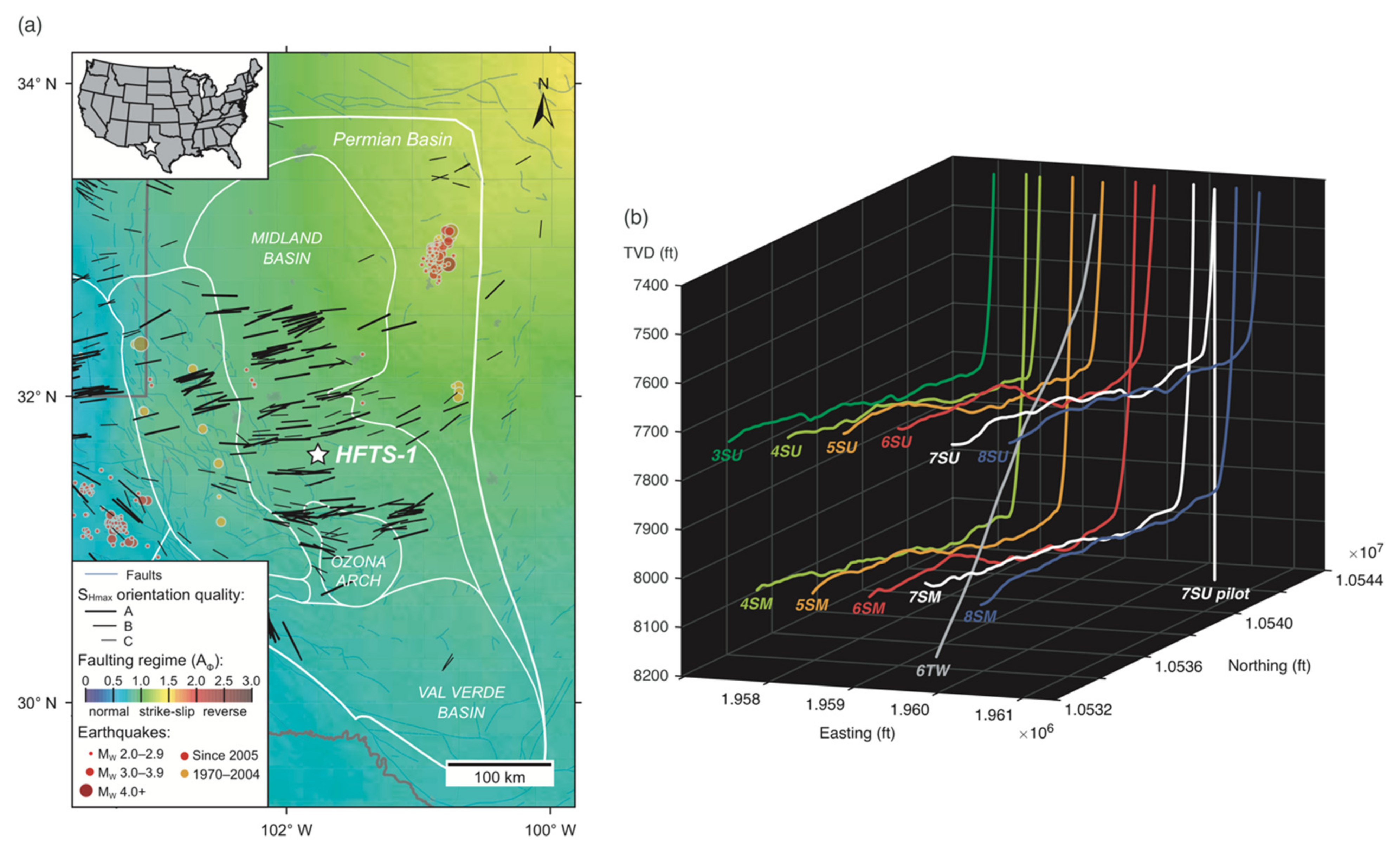
HFTS-1 is located within the Midland Basin in Western Texas (Figure 1a) [9]. In this region, the maximum compressive stress, SHmax, is oriented approximately E-W [10,11]. The background color in Figure 1a represents the value of the parameter Aϕ, which describes the ratio of the principal stress magnitudes:
where n = 0 for normal faulting, 1 for strike-slip faulting, and 2 for reverse faulting [12]. Based on the regional stress map, the Midland Basin is in normal/strike-slip faulting, so the vertical stress is the maximum principal stress, SV = S1; the maximum horizontal stress is the intermediate principal stress, SHmax = S2; and the minimum horizontal stress is the least principal stress, Shmin = S3. The value of Aϕ in the area of HFTS-1 is ~0.7.
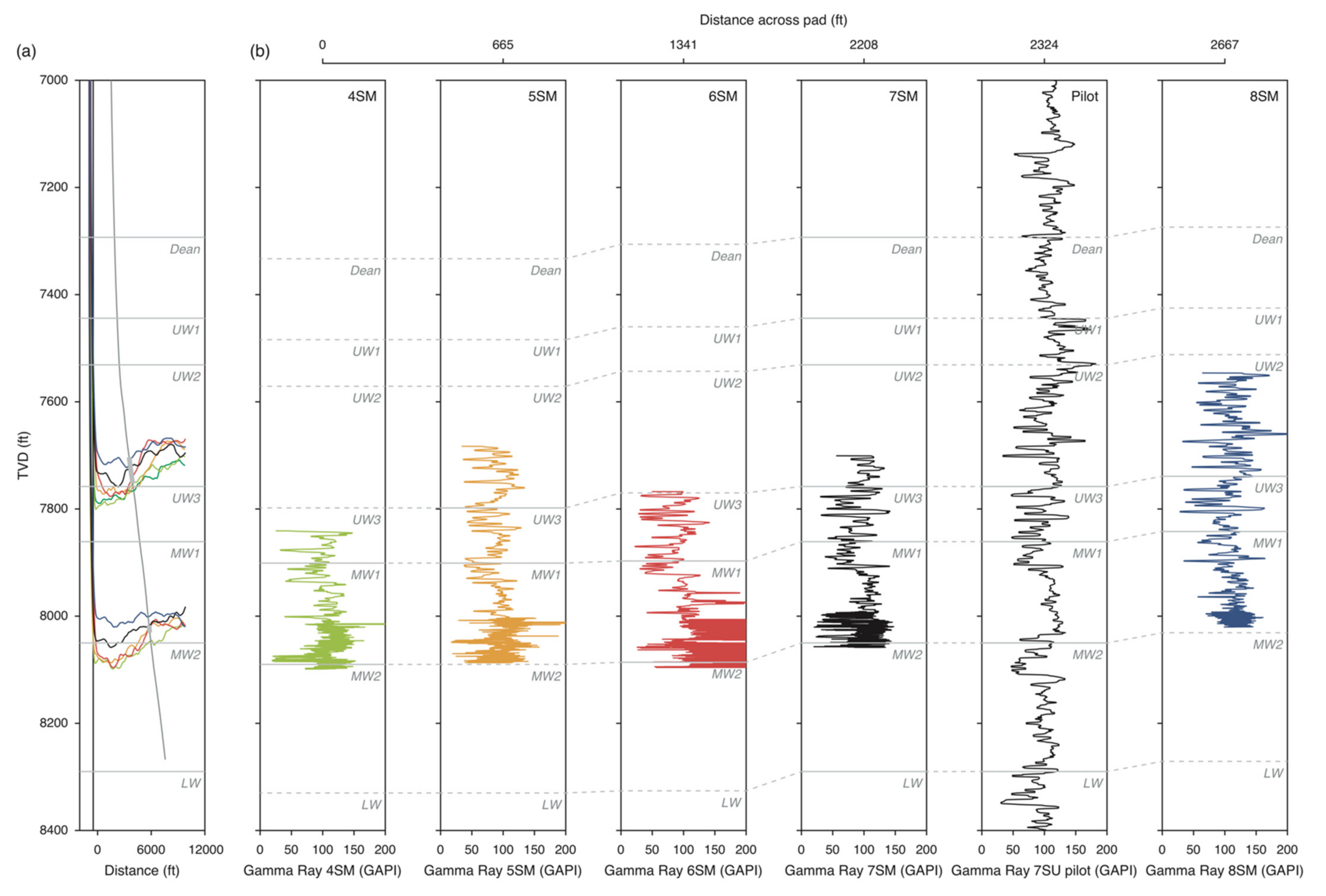
The HFTS-1 site comprises two sets of horizontal wells drilled N to S in a ‘wine rack’ pattern into the Upper and Middle Wolfcamp shale units (Figure 1b). A detailed stratigraphic description the Midland Basin is presented in U.S. Energy Information Agency reports on the Wolfcamp shale play [13]. There are six wells in the Upper Wolfcamp (UW) shale denoted by the suffix SU and five wells in the Middle Wolfcamp shale (MW) denoted by suffix SM. The number ID of each well denotes the pad from which it was drilled and increases from W to E. A vertical pilot well was drilled from pad 7 to a true vertical depth (TVD) of ~8500 ft (7SU pilot), and a number of well logs were collected: a Formation MicroImager (FMI) log to image fractures in wellbore, a Fourier transform infrared spectroscopy (FTIR) log to characterize mineralogy, a gamma ray log to identify stratigraphic boundaries, and a density log to estimate the overburden.
Each of the horizontal wells is ~10,000 ft long and was stimulated in 37–46 individual stages. Gamma ray logs were collected in all wells, but FMI logs were only collected in wells 6SU and 6SM. After each of the horizontal wells were hydraulically fractured and stimulated, a deviated well was drilled from pad 6 through the stimulated volume (6TW), and FMI logs and core samples were collected from two intervals, one within the Upper Wolfcamp (cores 1–4) and one within the Middle Wolfcamp (cores 5–6) (Figure 2a). During hydraulic fracturing and stimulation of each horizontal well, microseismic events were recorded by borehole geophone arrays in both vertical monitoring wells and neighboring horizontal wells [14].
2.2. Stress Measurements
In addition to well logs and core samples, diagnostic formation integrity tests (DFITs) were conducted to determine the magnitude of least principal stress, which in this case is the minimum horizontal stress (Shmin) (Appendix A Figure A1). During DFITs, a small hydraulic fracture is created, and then the well is shut-in for a period of days to months. The pressure decline curve is used to estimate stress, pore pressure, and formation permeability [15]. Six DFITs were collected in the 7SU pilot well, and DFITs were collected at the ‘toe’ of horizontal wells 4SU, 6SU, and 8SU in the UW and 6SM in the MW (Figure 2). Based on stratigraphic interpretation of gamma logs in the pilot well, the UW is subdivided into three units (UW1, 2, and 3), and the MW is subdivided into two units (MW1 and 2). We also determined the instantaneous shut-in pressure (ISIP) for each of the 434 hydraulic fracturing stages as a secondary estimate of Shmin. ISIPs are expected to be greater than Shmin by ~2–5 MPa due to contributions of perforation friction, near wellbore tortuosity [15], and stress shadow effects [16]. Since these effects are difficult to constrain, we only used the ISIPs support of the large scale variations in stress indicated by DFITs in different stratigraphic horizons.
3. Key Questions
3.1. Variations of the Least Principal Stress with Depth
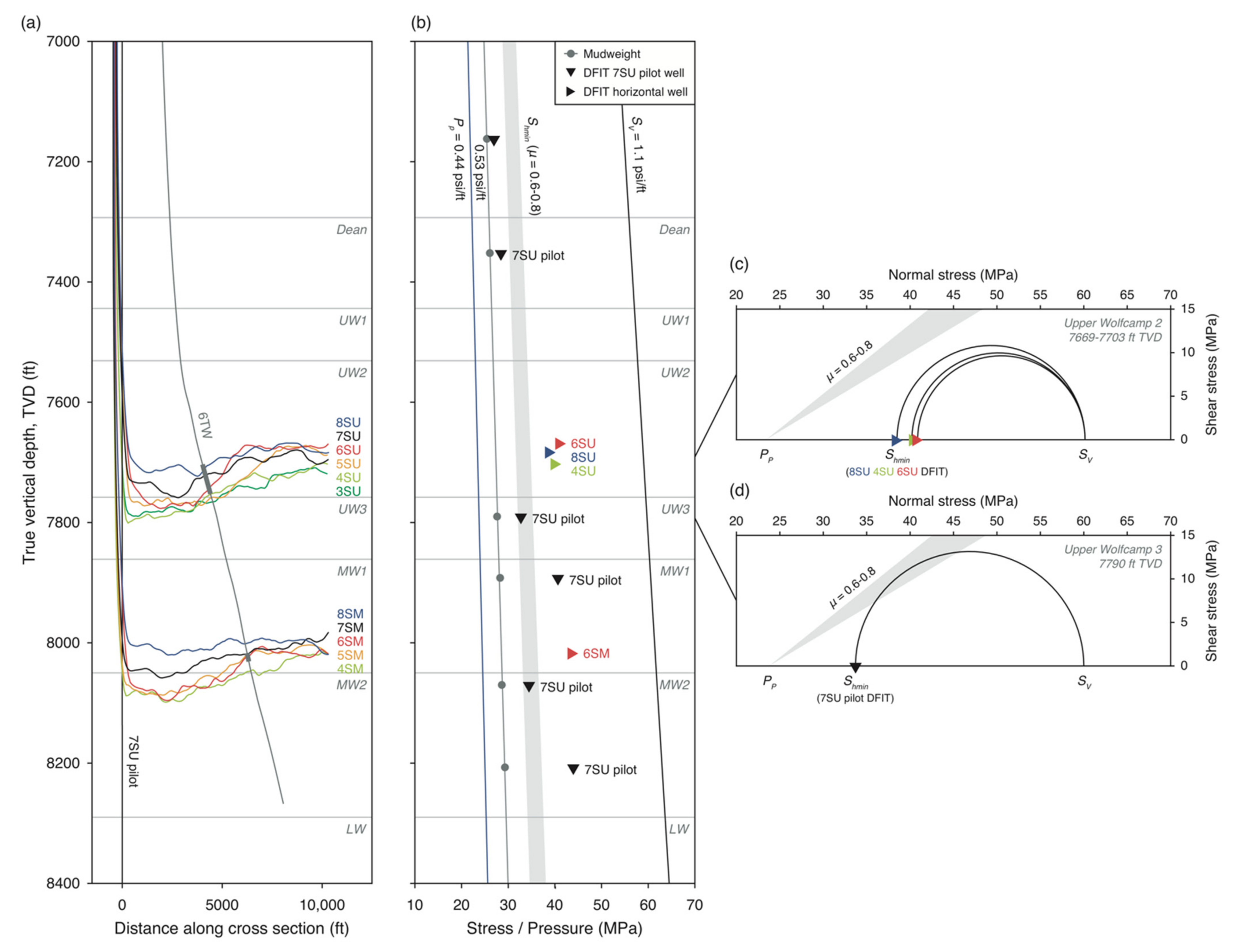
The horizontal wells in HFTS-1 are all drilled with a ‘toe up’ orientation (Figure 2a). In the UW, wells 3SU, 4SU, 5SU, and 6SU start in the UW3 and cross the boundary into the UW2, while wells 7SU and 8SU are only in the UW2. Similarly, in the MW, wells 4SM, 5SM, and 6SM start in the MW2 and cross the boundary into the MW1, while wells 7SU and 8SU are only in the MW1.
Figure 2b shows a vertical profile of stress and pore pressure in the reservoir. The drilling mudweights were recorded at the true vertical depth (TVD) of each DFIT measurement in the pilot well and show a mudweight gradient of ~0.53 psi/ft, not significantly greater than the hydrostatic pore pressure gradient, 0.44 psi/ft. This indicates that wells were drilled in nearly a ‘balanced’ fashion, so we considered the mudweight as an upper bound on the in situ pore pressure. The vertical stress gradient, 1.1 psi/ft, was determined by integrating the density log from the vertical pilot well. DFIT measurements in the Dean and overlying Lower Sprayberry units show Shmin values slight lower than those predicted by frictional equilibrium for the range friction coefficients expected in unconventional reservoir rocks, μ = 0.6–0.8 [17]. In the UW, DFIT measurements in the horizontal wells and pilot well reveal significant variations as a function of depth. In the UW2, DFIT values decrease with increasing TVD from well 6SU to 4SU. This pattern appears to continue into the UW3, where a DFIT measurement in the vertical pilot well is consistent with the value of Shmin predicted by frictional equilibrium. In the MW, DFIT measurements indicate that the Shmin is above frictional equilibrium in the upper part of the MW1 and increases with depth, then decreases to a value consistent with frictional equilibrium in the MW2, then increases again at the base of the MW2.
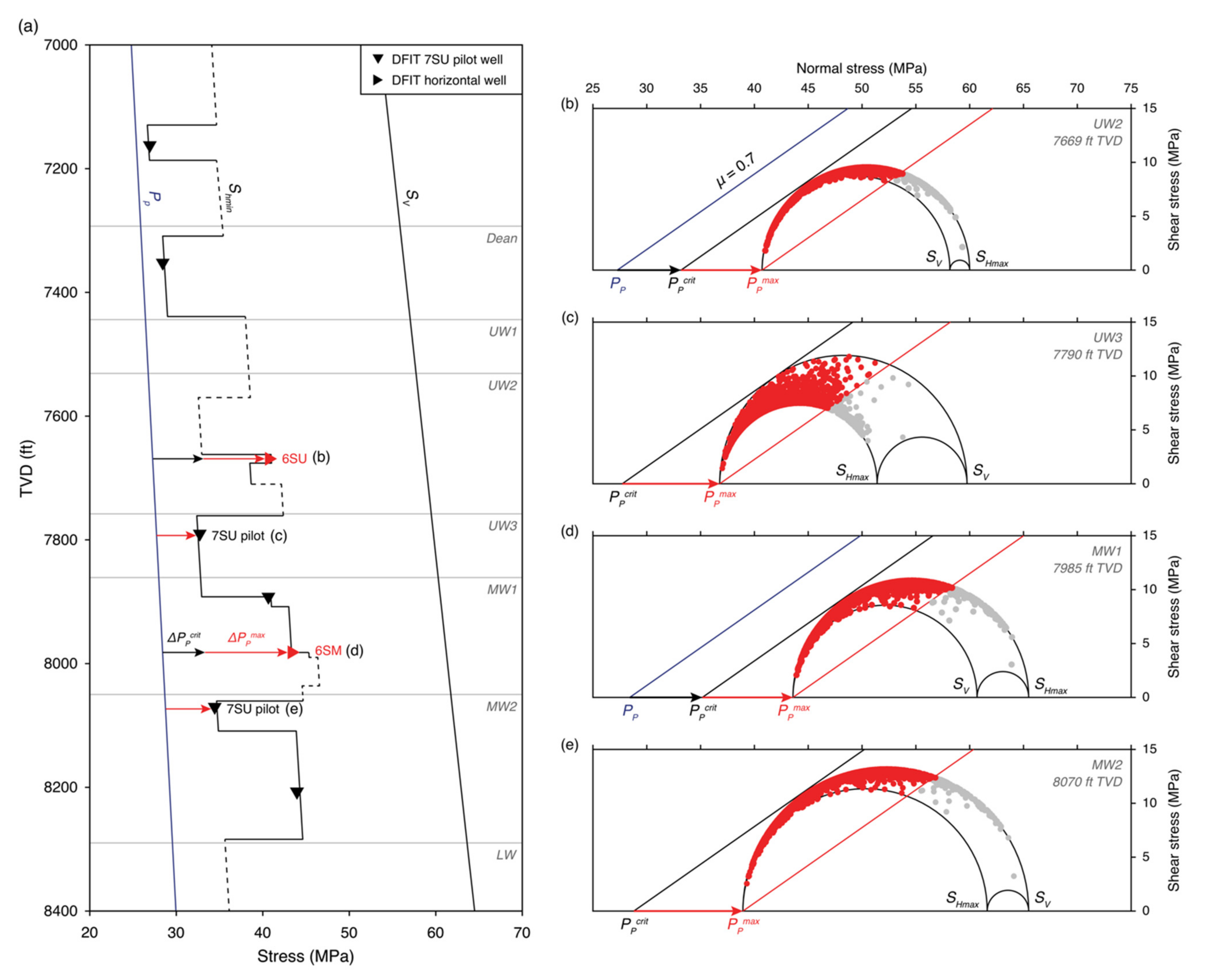
The variations in Shmin captured by the DFITs can be represented by 2D Mohr circle diagrams in terms of frictional faulting theory (Figure 2c,d). The half circle represents the values of shear and normal stress resolved on faults of varying orientations. In a normal/strike-slip faulting regime, the differential stress is, S1 − S3 = SV − Shmin. In the UW2, as differential stress decreases with depth from well 6SU to 4SU over ~30 ft, the Mohr circle moves closer to the frictional equilibrium line (Figure 2c), while ~90 ft below in the UW3, the differential stress is consistent with frictional equilibrium (Figure 2d). The first goal of this study is to try to explain this stress stratigraphy in terms of rock properties.
3.2. Impact of Stress Variations on Hydraulic Fracture Growth and Microseismicity
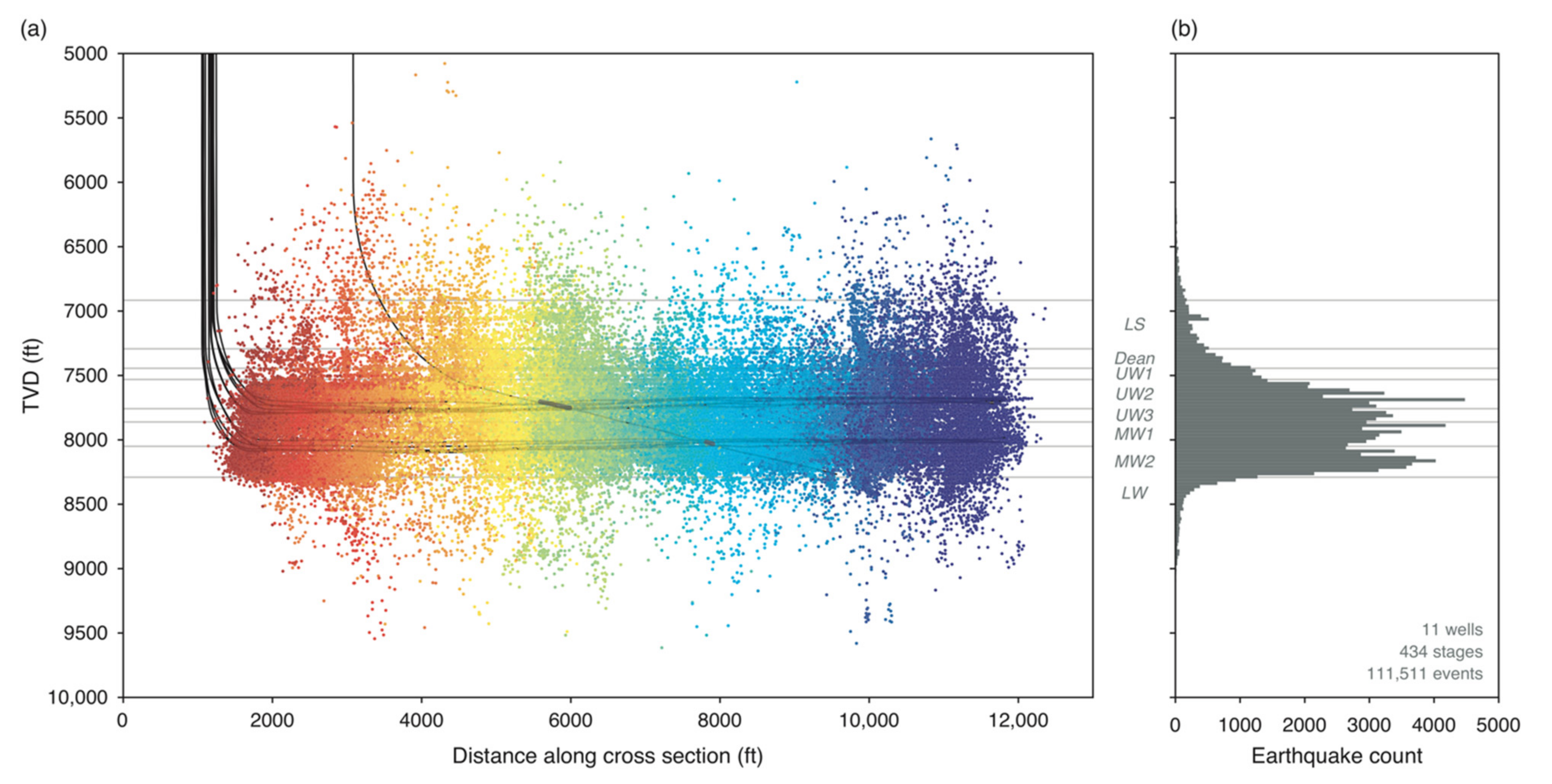
The second goal of this study is to determine how variations in stress with depth impact vertical hydraulic fracture growth and slip on pre-existing faults. Figure 3a shows a N-S cross section of the HFTS-1 wells with >100,000 recorded microseismic events, which are colored by the hydraulic fracturing stage from which they were generated. While it is difficult to see any patterns in the event locations across the length of the horizontal wells, it is clear there are some lateral variations in the vertical extent of seismicity, which indicates how far fluid pressure from hydraulic fractures leaks off to pre-existing faults. Figure 3b shows a histogram of the microseismic events. While difficult to see any patterns as a function of depth, the majority of events appear to be contained between the UW1 and LW boundaries. Our goal is to use the observed patterns of microseismicity in space and time to interpret the impact of stratigraphic stress variations on hydraulic fracture growth.
4. Constructing a Profile of the Least Principal Stress
DFITs provide a partial picture of the stress profile, but in order to interpret the value of Shmin in regions with no stress measurements, we need to understand what gives rise to the observed stress stratigraphy. A number of recent studies have used the theory of viscoplastic stress relaxation to account for values of Shmin above what is predicted by frictional equilibrium [3,6,7]. In this framework, rocks with high viscous compliance are able to relax differential stress over time, which, in a normal faulting stress regime, equates to the value of Shmin increasing with respect to SV.
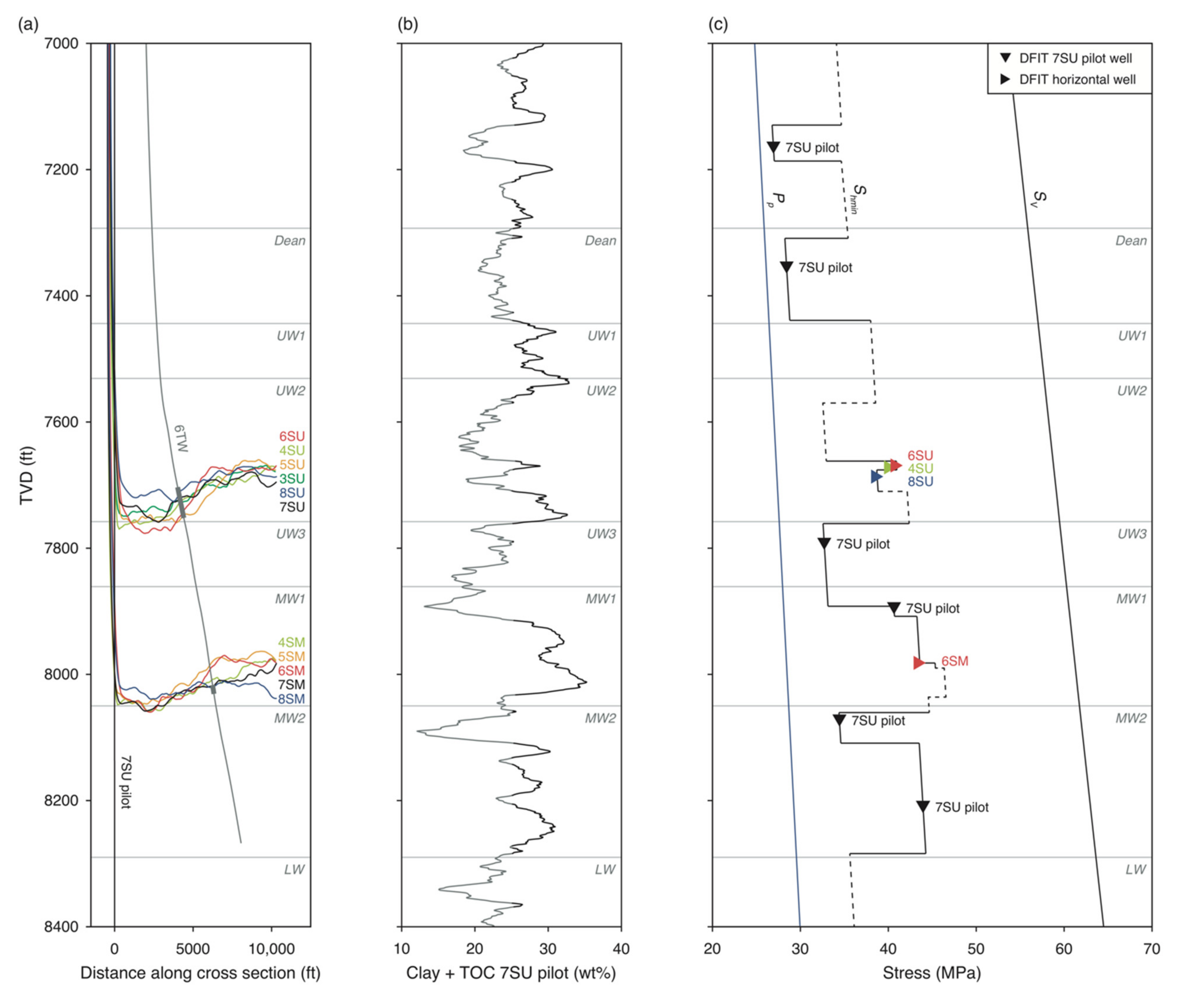
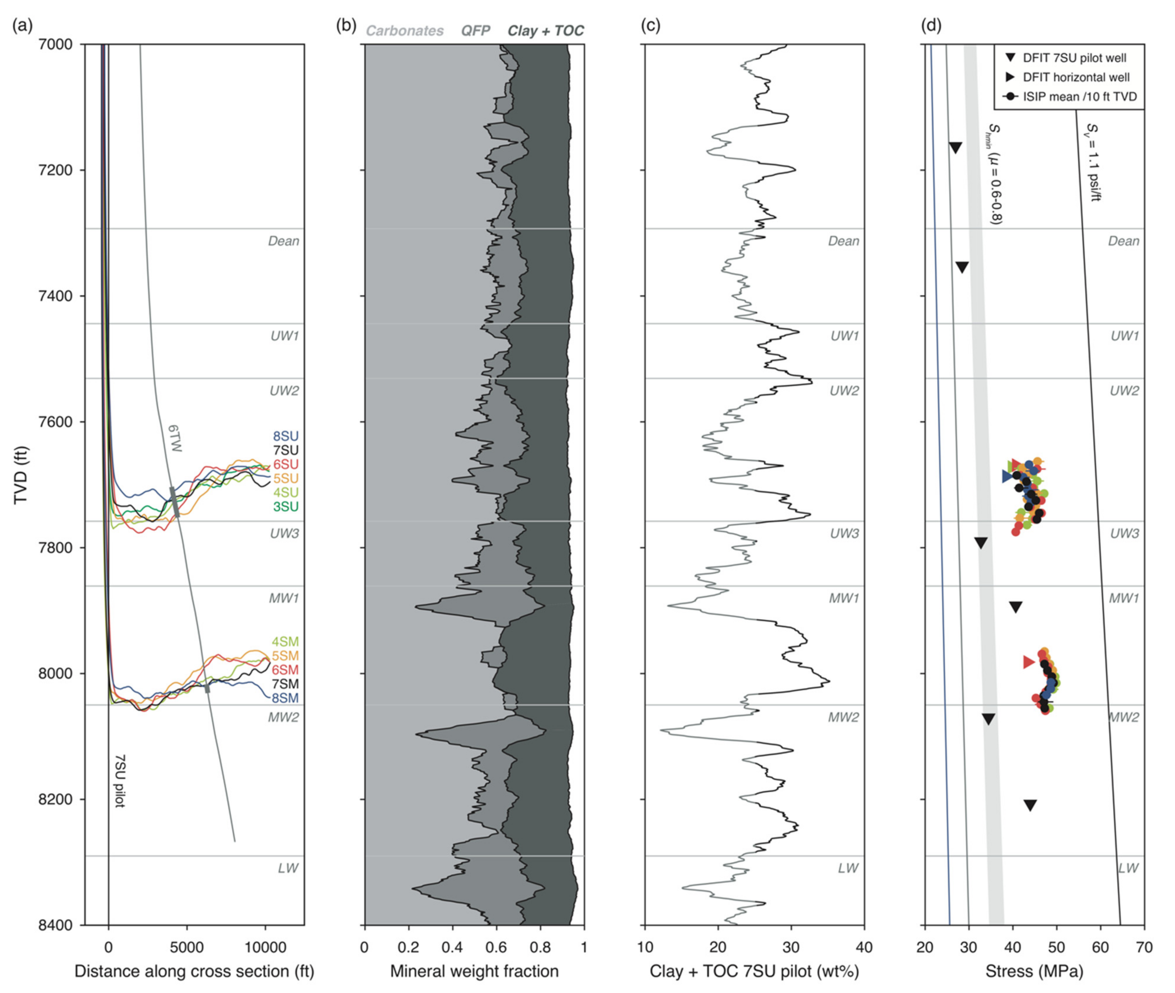
Laboratory creep experiments indicate that the primary controls on viscoplastic stress relaxation are rock microstructure and composition, specifically the quantity of clay minerals and total organic carbon (clay + TOC). Clays and organic deposits are more porous and compliant than carbonates or silicates, so more stress is relaxed over time in clay + TOC-rich rocks. Figure 4b shows the variation in clay + TOC as a function of depth in the 7SU pilot well from a mineralogy log derived from Fourier transform infrared spectroscopy (FTIR) measurements. A median filter is applied remove high frequency noise. Note that clay + TOC varies significantly across the Wolfcamp strata from ~10–35 wt%.
Comparing the clay + TOC log to the DFIT values from the 7SU pilot well reveals a clear pattern: Regions with relatively low clay + TOC (<25 wt%) show relatively high differential stress, with Shmin values below or consistent with frictional equilibrium (e.g., LS, Dean, UW3, and top of MW2), while regions with clay + TOC values above this threshold show relatively low differential stress, with Shmin values above frictional equilibrium (e.g., MW1 and base of MW2) (Figure 4c).
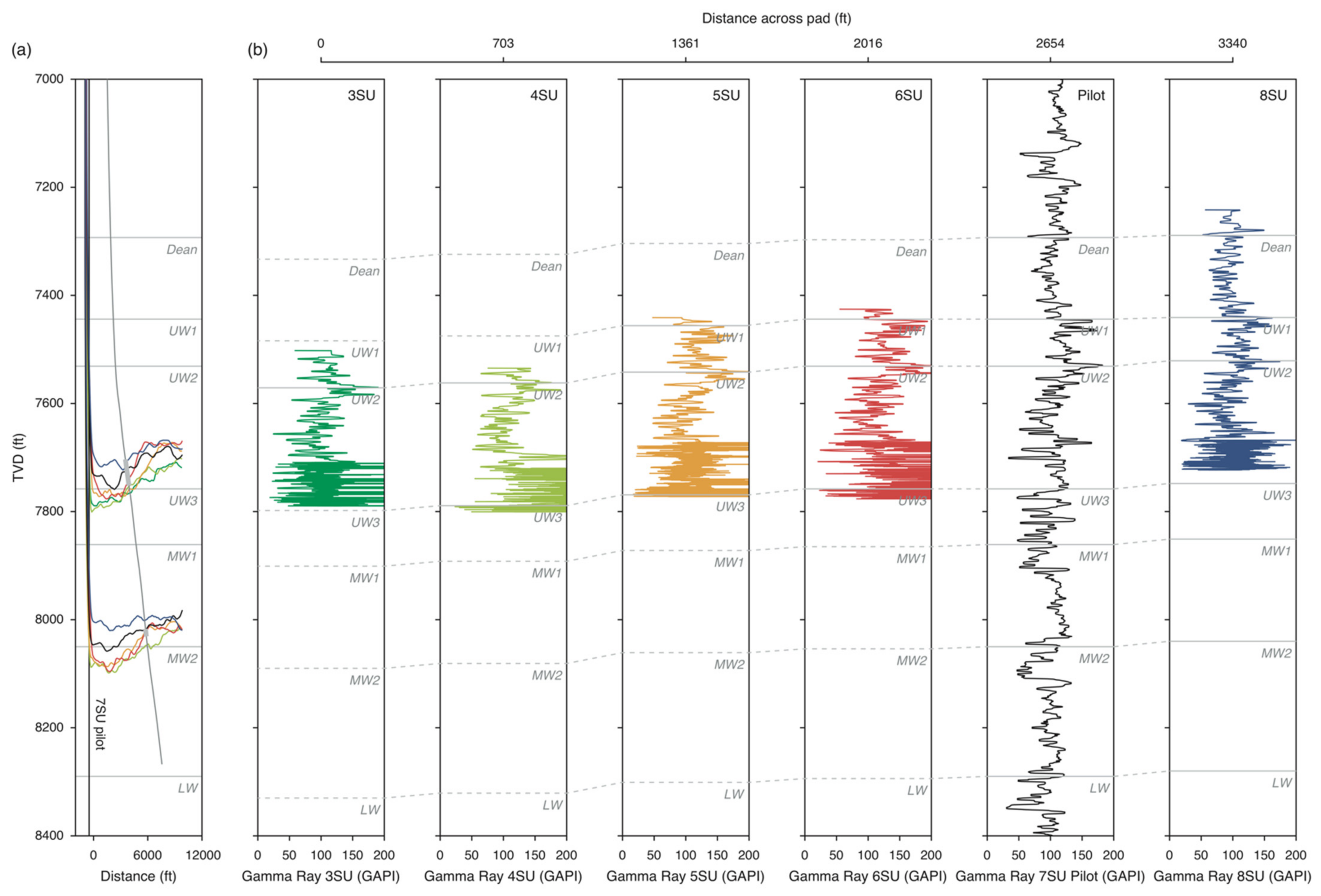
To compare the DFIT values from the horizontal wells to the compositional log from the 7SU pilot well, we need to account for variations in vertical stratigraphy across the HFTS-1 pad. By comparing the gamma logs from each horizontal well to vertical pilot well, we determined the TVD difference between the tops of each stratigraphic unit. We then used this information to shift the DFIT from each horizontal well, such that they are consistent with the stratigraphy of the pilot well. The magnitude of this shift increases from E-W as the stratigraphy deepens (Figure A2 and Figure A3). The largest difference in stratigraphy occurs in wells from pads 3 and 4, in which the formation tops are ~40 ft deeper than in the pilot well. After shifting each of the horizontal well DFITs, the values appear consistent with the pattern in the pilot well, even tracking higher frequency variations in clay + TOC (e.g., 7650–7700 ft TVD).
As Shmin appears to be strongly correlated with clay + TOC, we constructed an interpreted stress profile that accounts for the stratigraphically shifted stress measurements (solid lines) and extrapolates the pattern of viscous stress relaxation in high clay + TOC strata over the entire stratigraphic section (dashed lines) (Figure 4). We assume that the low clay + TOC strata are in frictional equilibrium, with a friction coefficient of μ = 0.7, and that the high clay + TOC strata follow the DFIT values. In the high clay + TOC strata with no stress measurements (e.g., base of LS and UW1), we used vertical distribution of microseismic events to constrain of the estimated value of Shmin, which is discussed in detail in Section 5. ISIP values from hydraulic fracturing stages confirm the large scale variations shown by the DFITs in different stratigraphic horizons (Figure A4). In Section 6, we use the ISIPs from groups of stages in the same strata to interpret differences in vertical hydraulic fracture growth and the characteristics of induced microseismic events.
5. Impact of Stress Variations on Vertical Hydraulic Fracture Growth
We used the Shmin profile (Figure 5a) based on lithological variations (Figure 5b) to interpret the patterns of vertical hydraulic fracture growth across the length of the horizontal wells. For the purposes of this paper, we focus on observations from well 6SU, which crosses the UW2/UW3 boundary (~7750 ft TVD), and well 6SM, which crosses the MW1/MW2 boundary (~8050 ft TVD) (Figure 4a).
After stratigraphically shifting the well trajectory into the pilot well reference frame, well 6SU slightly crosses into the UW3 at its deepest stages (Figure 5c). Over the ~50 ft TVD from heel to toe, the clay + TOC is expected to increase from ~20 to ~30 wt%. Five toe stages show instantaneous shut-in pressure (ISIP) values consistent with the DFITs, noting that the ISIP values are likely greater than Shmin by ~2–5 MPa. The five deepest stages near the heel show lower ISIP values, consistent with what we expect based on the change in lithology.
The vertical distribution of microseismic events in these two groups of stages appears to be controlled by the predicted variations in Shmin (Figure 5c). In the heel stages, microseismic events are concentrated in the UW3 and extend upwards to the base of the UW1 and downwards to the MW2. In contrast, the events in the toe stages are concentrated within the MW1/MW2 and extend upwards into the LS and downwards into the LW. In addition, the toe stages show a more events overall and many more events in the target formation, the UW2 (Figure 5d).
The difference in the vertical extent and number of microseismic events between the heel and toe stages can be simply understood in terms of the interpreted stress profile. In the heel stages, pore pressure can only be raised to the relatively low value of Shmin (~40 MPa); however, since this value is greater than stresses in the UW2 above and greater than the UW3 below, hydraulic fractures can propagate both upwards and downwards, delivering the fluid pressure needed to induce slip on fault. The fact the microearthquakes in the heel stages are limited vertically by the MW1 signifies that there must be an even higher stress barrier in that unit, which is consistent with the high clay + TOC values in that strata. In the toe stages, pore pressure can be raised further (~48 MPa), and the fact that seismicity extends both upwards and downwards with no apparent barriers indicates that this difference in stress is enough to allow hydraulic fractures generated in the toe to propagate through both the high stress barriers that appear to limit the vertical extent of seismicity in the heel stages. In addition, because the pore pressure can be raised further in the toe stages, we expect more faults that are not optimally oriented in the present stress field to slip, which likely explains why more events are observed in the toe compared to the heel overall. Based on these observations, we interpreted the value of Shmin in the UW1 to fall between the ISIP values of the heel and toe stages (~45 MPa) and posit that a similar stress barrier may exist within the LW at ~8400 ft.
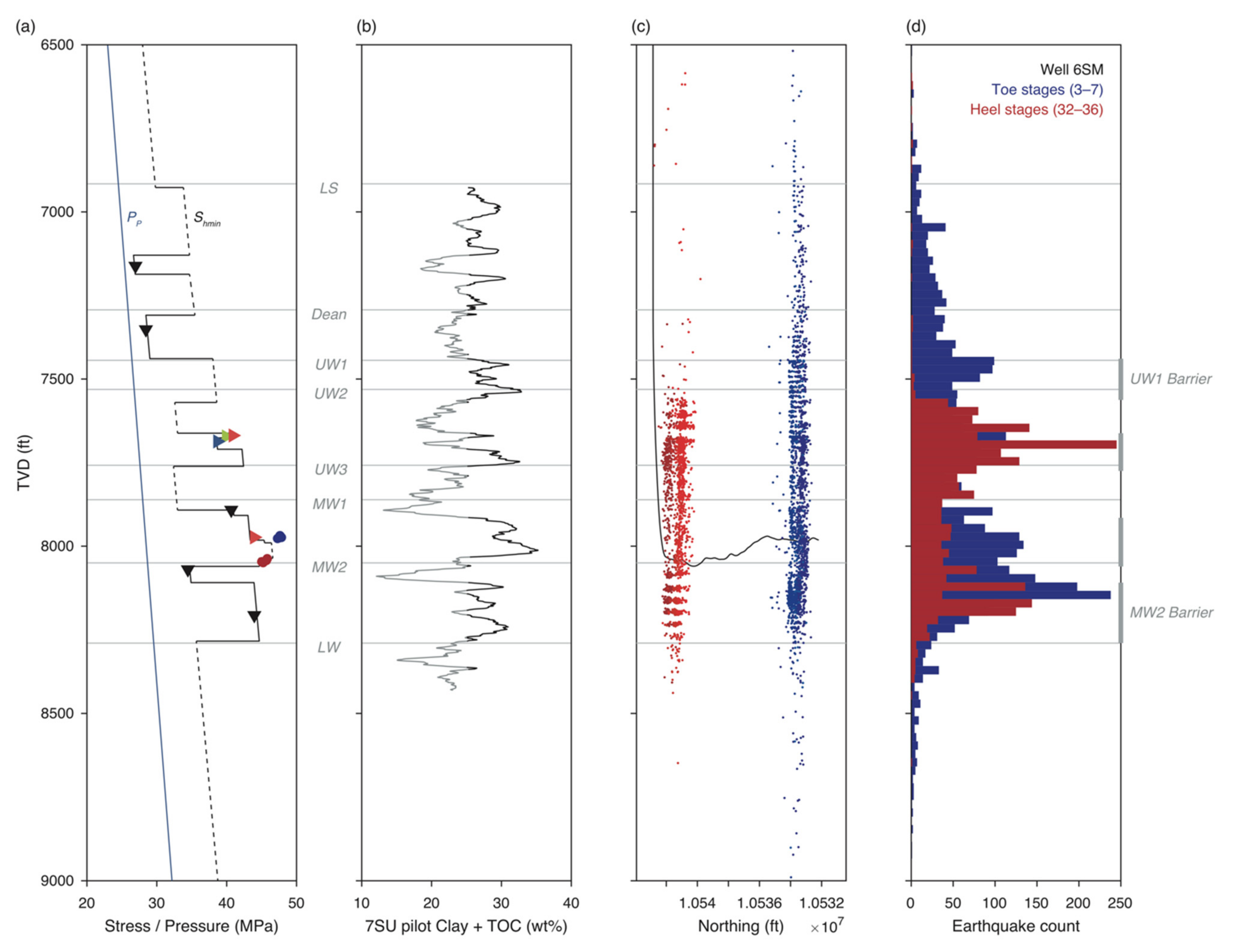
We performed a similar heel to toe comparison in well 6SM across the MW1/MW2 stratigraphic boundary, focusing on stages 32–36 in the heel at the base of the MW1 and stages 3–7 near the toe (Figure 6). The microseismic events in the heel stages are concentrated in the UW2 and extend upwards to the base of the UW1 and downwards to into the LW. In contrast, the events in the toe stages are concentrated within the MW2 and extend upwards into the LS and much deeper into the LW. Similar to well 6SU, the toe stages show a much greater number of events and many more events in the target formation, the MW.
We can also make sense of patterns of microseismicity along well 6SM in terms of the interpreted stress profile. In the heel stages, pore pressure can only be raised up to the value of Shmin (~45 MPa); however, since this value is greater than stresses in the UW2 and UW3 above and greater than the MW2 below, hydraulic fractures can propagate both upwards and downwards, which explains the observed pattern of microseismic events. The fact the events in the heel stages are limited vertically by the UW1 confirms that there must be an equal or greater stress barrier in that unit. By the same logic, there must also be a higher stress barrier within the LW, approximately at the base of pilot well where the clay + TOC log ends. In the toe stages, pore pressure can be raised only slightly higher (~48 MPa); however, the fact that seismicity extends both upwards and downwards with no apparent barriers indicates that this small difference in stress is enough to allow hydraulic fractures generated in the toe to propagate through the stress barriers that limit the vertical extent of seismicity in the heel stages. As in well 6SU, the higher pore pressure needed in the toe stages allows poorly oriented fault slip, resulting in many more events in the target formation. The variations in stress and seismicity across both wells 6SU and 6SM are consistent with the interpreted stress profile and indicate that the major stress barriers are the UW1, MW1, and possibly the LW at ~8500 ft.
6. Fracture Analysis
The next step in understanding the observed patterns of stimulation is examining the population of faults and fractures that may slip when fluid is injected.
6.1. Fracture Observations
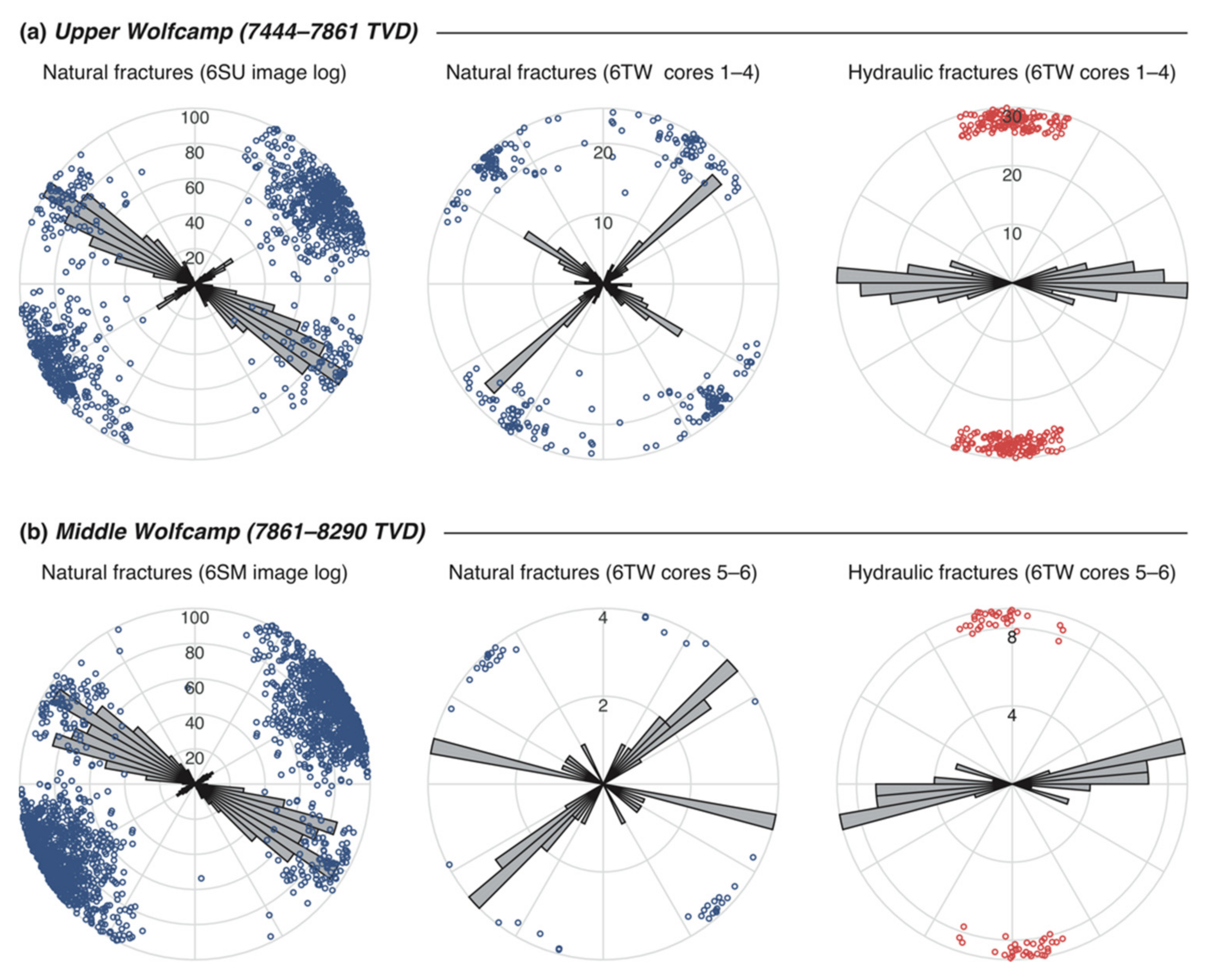
Pre-existing fractures at HFTS-1 are documented in image logs in wells 6SU, 6SM, and 7SU and the post-stimulation core recovered in well 6TW. A detailed description of the core and fractures are provided by Gale et al. (2018) and Elliot and Gale (2018) [18,19]. Figure 7 shows the fracture data in the UW and MW units. Image logs in both horizontal wells reveal a consistent set of steeply dipping, conjugate fractures, with the primary population striking NW. A similar distribution of natural fractures is also observed in the core samples from well 6TW [19]. In addition to the natural fractures, E-W striking hydraulic fractures are also observed in post-stimulation core. Hydraulic fractures are expected to form parallel to SHmax, so these fractures are consistent with the approximately E-W regional stress direction determined by wellbore stress orientation measurements (Figure 1a).
6.2. Impact of Stress Variations on Induced Shear Slip
We applied the interpreted stress profile to the fracture data to determine what fracture orientations can slip when pore pressure is increased during hydraulic stimulation (Figure 8). We used the DFIT measurements of Shmin (Figure 4c) in conjunction with observations of wellbore failure to constrain the value of SHmax (Figure A6). To illustrate the impact of stress variations on the potential for fault slip, we constructed Mohr circle diagrams (Figure 2) for Upper Wolfcamp (UW) and Middle Wolfcamp (MW) strata that represent high stress barriers (Figure 8c,e) and for strata that are in frictional equilibrium (Figure 8b,d). On each Mohr circle, the population of fractures represents the sum of all natural fracture observations the given strata. We defined two threshold pore pressure values for stimulation. PPcrit is the pore pressure need to induce slip on critically stressed faults given a coefficient of friction of 0.7, and PPmax is the pore pressure needed to propagate the hydraulic fracture, i.e., Shmin.
In the MW, the MW1 is a high stress barrier, so in order to stimulate slip on pre-existing faults, the pore pressure needs to be raised by more than 20 MPa, more than any other layer (Figure 8d). This explains why hydraulic fractures generated in the SM wells can propagate through the less effective stress barriers above and below. In contrast, the top of the MW2 is in frictional equilibrium, so any small increase in pore pressure would induce slip on well-oriented faults (Figure 8e).
7. Impact of Stress Variations on Microseismicity
Microseismic events are an important tool for understanding the stimulation process because they provide direct evidence that fluid pressure was raised to a critical value at a certain distance from the injection point at a certain time. However, the cloud of microseismic events should not be misinterpreted as a proxy for the stimulated reservoir volume or the hydraulic fracture area. Rather the spatiotemporal distribution of events should be used in context of the stress profile to interpret differences in the fracturing and stimulation process.
7.1. Spatiotemporal Distribution of Events
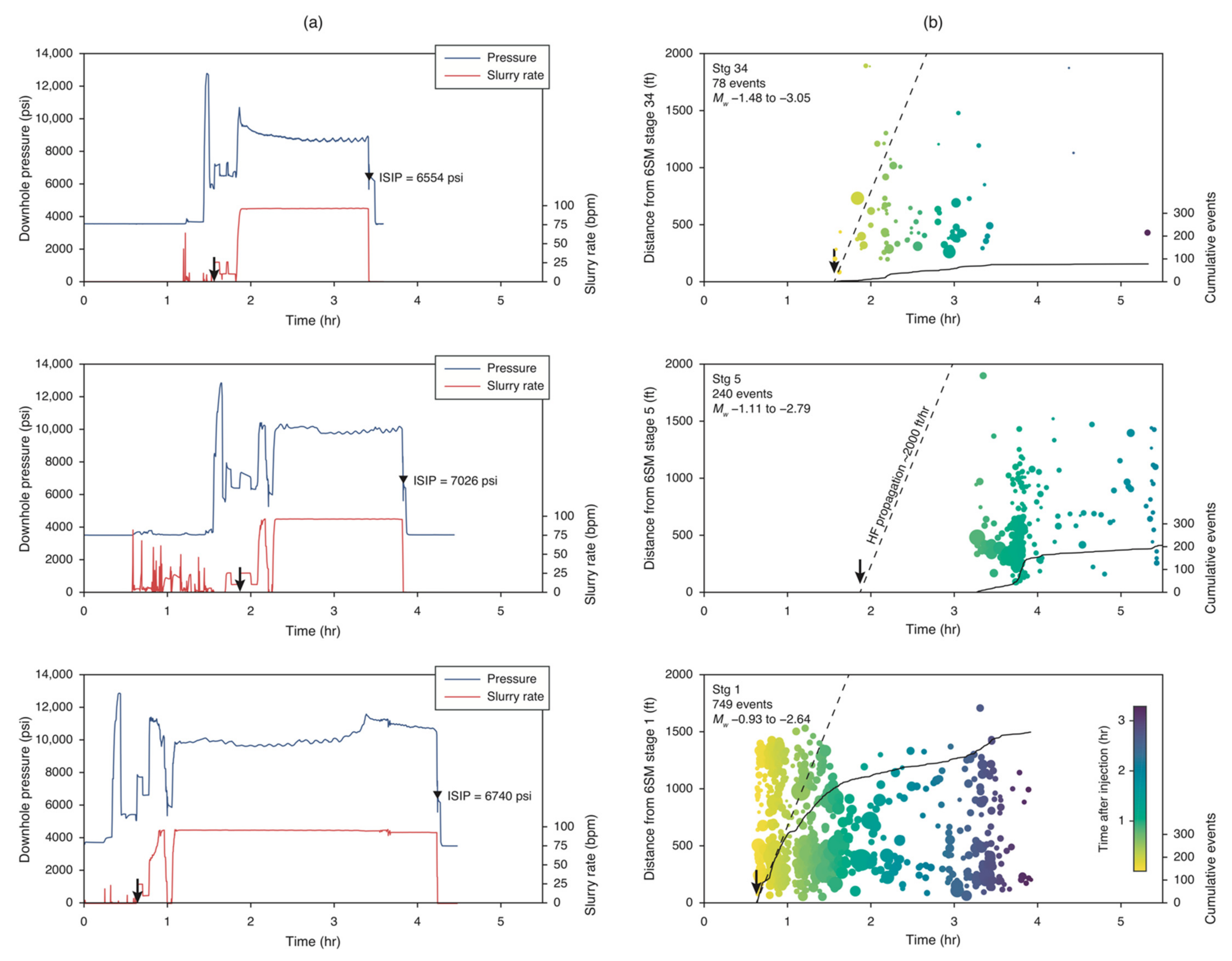
For this study, we focused on microseismic data from well 6SM, which shows significant variations in composition, stress, and the vertical extent of seismicity between the heel and toe stages (Figure 6). Comparing the pumping record and spatiotemporal distribution of microseismic events (Figure 9 and Figure 10) reveals several characteristic stimulation responses.
Stage 34 near the heel has a relatively low value of Shmin, close to what is predicted from frictional equilibrium. Microseismic events are induced instantaneously upon the start of pumping and propagate away from the well at approximately the expected rate of hydraulic fracture propagation (~2000 ft/h). This indicates that pore pressure only needed to be raised slightly to trigger slip on well-oriented faults (Figure 8e). Therefore, any leak-off from the hydraulic fracture would induce slip on faults in this relatively low stress strata. The microseismic events also appear limited above by the interpreted high stress layer in the UW1 and below by the interpreted high stress layer in the LW. This is consistent with our estimate of the stress being close to frictional equilibrium, as pressure to propagate a hydraulic fracture in this low stress strata is not sufficient to do so in the high stress layers above and below.
Stage 5 near the toe has a high value of Shmin consistent with the 6SM DFIT. In contrast to Stage 34, microseismic events are only induced over an hour after the start of pumping. This is consistent with the high value of Shmin because the pore pressure has to be raised significantly to induce slip on even well-oriented faults (Figure 8d). Since slip on faults is induced by leak-off into the low permeability matrix, even after the fracture forms, it takes time for the pressure on faults to be raised enough for slip to occur. Similar patterns have been observed in a recent case study from the Niobrara shale [8]. Because pore pressure needs to be raised significantly to propagate a hydraulic fracture in this high stress layer, the resulting fracture can also propagate through the lower stress layers above and below and can induce shear slip within those layers (e.g., UW1 and MW2).
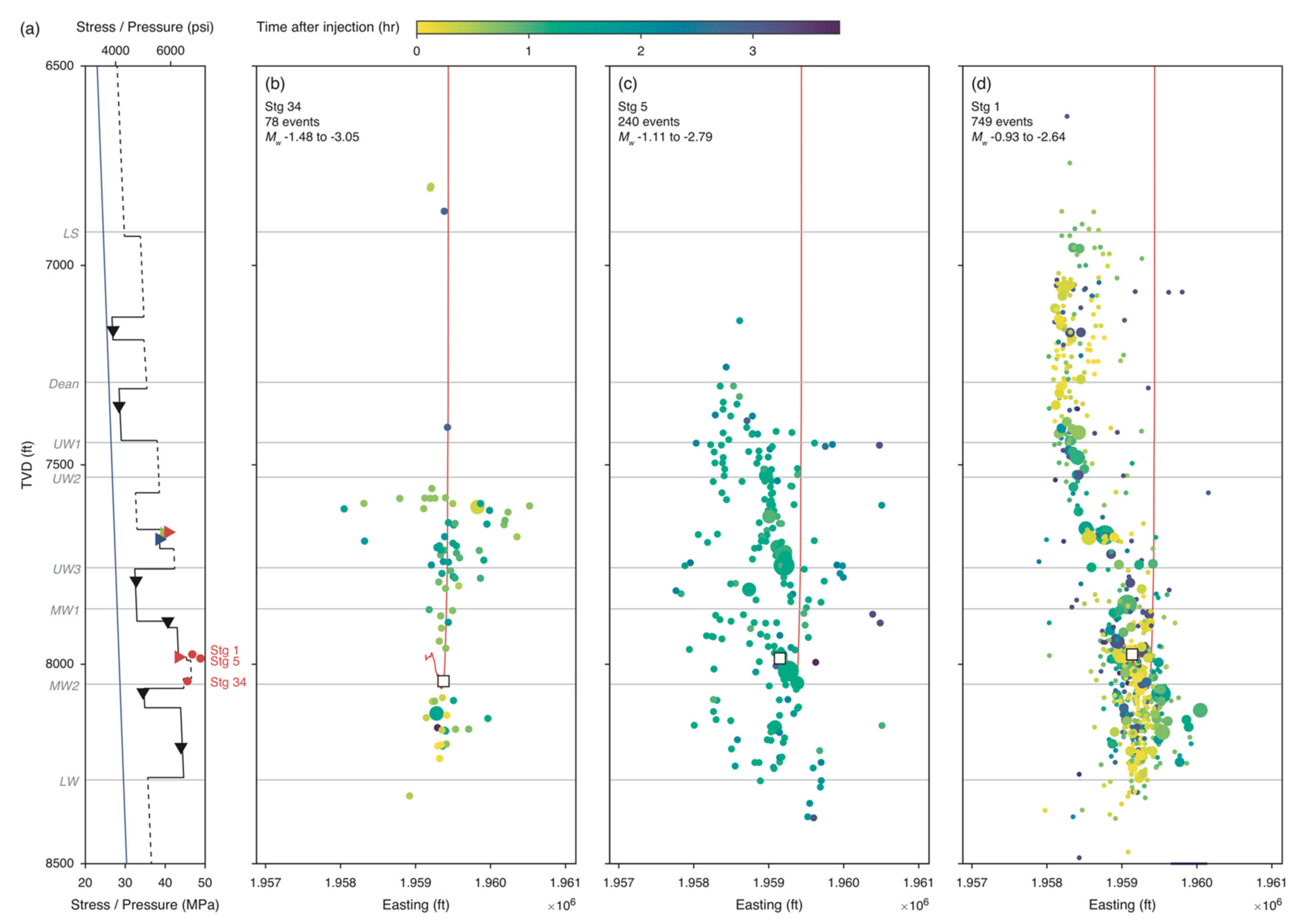
Stage 1 also has a high value of Shmin, but there is no delay in the onset of microseismic events. Events are induced instantaneously upon the start of pumping and quickly propagate upwards and away from the well into the LS, faster than the expected propagation velocity of a hydraulic fracture. These early time events can be fit in 3d space by a steeply dipping plane, striking obliquely to SHmax (Figure 10c), consistent with the orientation of critically stressed natural fractures (Figure 7). Therefore, we hypothesize that the hydraulic fracture in this stage directly intersected a well-oriented, pad-scale fault, which transported fluid pressure upwards quickly, generating events on well-oriented fractures on intersecting strands or within the fault damage zone. Because the hydraulic fracture was directly connected to the fault, no time was needed to raise the pore pressure to the critical value, unlike in Stage 34, where the events were induced at an early time by leak-off from the hydraulic fracture.
7.2. Source Mechanisms
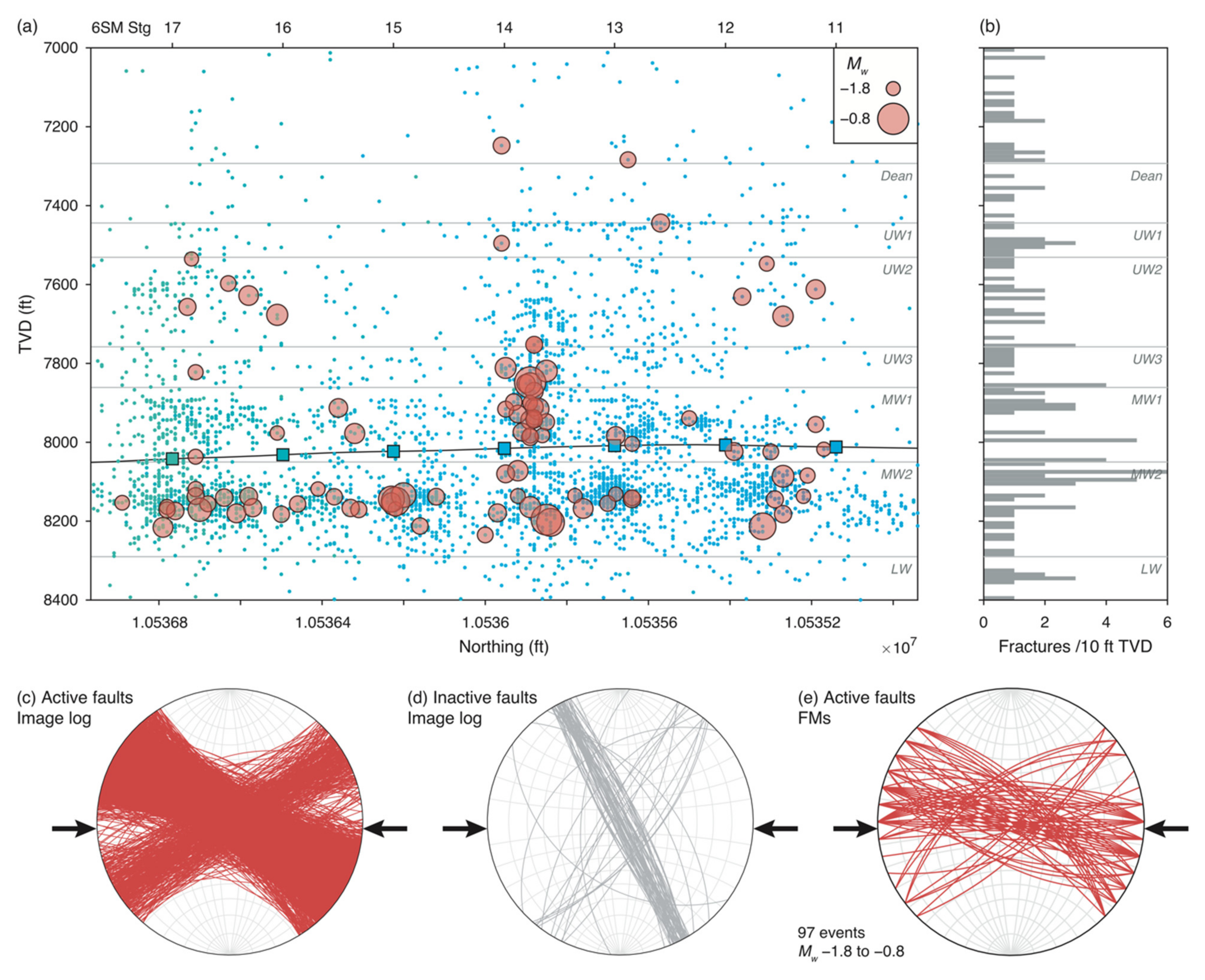
To further explore the relationships between the stress stratigraphy and microseismicity, we determined the source mechanisms for a population of larger events (>Mw − 2.0) from well 6SM, stages 11–17 (Figure 11). Moment tensor solutions were obtained by invert microearthquake focal mechanisms using the software package MicroFM [20]. Figure 11a shows the distribution of microseismic events and select events with moment tensor solutions. All events are colored by stage (Figure A5), and events with moment tensor solutions are plotted red and sized by magnitude. The moment magnitude, Mw, range for the events with moment tensor solutions is approximately −1.8 to 0.8. Figure 9b shows fracture counts/10 ft TVD interval from the vertical pilot well. The relatively dense cluster of fractures within the MW may in part explain why more and larger events are generated in the MW than the overlying or underlying layers.
Figure 11c–e compares fractures planes observed in image logs with the primary nodal planes from the focal mechanism (FM) inversion. The primary nodal planes are generally consistent with the orientation of fractures observed in image logs are well-oriented for normal/strike-slip faulting given the E-W orientation of SHmax indicated by hydraulic fractures in the core (Figure 7).
The microseismic source mechanisms can also provide further insight into the stimulation process in terms of the timing of the events. We focused on five events (ordered by time) with moment tensor solutions in well 6SM, stage 14 (Figure 12). Events 1, 2, 4 represent normal/strike-slip motion on well-oriented faults. Events 1 and 2 are relatively close to the well and occur at an early time, and event 4 is relatively far away and occurs later. All these events fall close to the line representing hydraulic fracture propagation, indicating that they were likely generated by leak-off from the hydraulic fracture when it reached the given distance. Events 3 and 5 represent normal motion on poorly oriented faults oriented sub-parallel to SHmax. Event 3 is relatively close to the well but falls off the hydraulic fracture propagation line, indicating that that additional time was needed for leak-off or for the hydraulic fracture to grow near enough to the fault region to raise the fluid pressure. Event 5 is actually the closest to the stage but occurs at the latest time because it is the least well-oriented for slip in the stress field.
8. Conclusions
Based on well logs, core data, microseismicity, and stress measurements, we constructed a geomechanical model for HFTS-1 that accounts for stratigraphic variations in rock properties and stress. Strata with high clay + TOC show high values of the minimum horizontal stress, Shmin (low differential stress), consistent with the theory of vicous stress relaxation, while strata with low clay + TOC show values of Shmin consistent with frictional faulting theory. We used the stress profile in conjunction with fracture data and the observed distribution of microseismic events to demonstrate that vertical hydraulic fracture growth is controlled by stratigraphic variations in Shmin. We also determined microseismic focal mechanisms for select microearthquakes and showed that the spatiotemporal distribution of events can be explained by the stress model.
The conceptual framework developed here shows that accounting for viscous stress relaxation in layered sequences is essential for controlling hydraulic fracturing and injection-induced microseismicity. In unconventional reservoirs, which have considerable variations in mineralogy and rock properties, it essential to understand what gives rise to stress relaxation in order to focus stimulation (increase surface area) within the most production zones. Our results also have several important implications for energy production and storage in geologic reservoirs:
- (1)
- To compare logs, core data, and stress measurements from different wells, data must be shifted into a single stratigraphic reference frame.
- (2)
- Hydraulic fracturing stage ISIP values reflect large-scale stress variations shown by DFITs.
- (3)
- Stratigraphic variations in Shmin are a primary control on vertical hydraulic fracture growth. Strata with high values of Shmin (low differential stress) may act as a barriers to either upward or downward growth.
- (4)
- Stratigraphic variations in Shmin control the amount of pressure needed for stimulation and thereby determine the quantity, orientation, and spatiotemporal distribution of microseismic events.
- (5)
- Horizontal wells passing through stratigraphic boundaries can result in variable stimulation outcomes.
Author Contributions
Conceptualization, A.K. and M.Z.; methodology, A.K.; software, A.K.; validation, A.K. and M.Z.; formal analysis, A.K.; investigation, A.K.; resources, M.Z.; data curation, A.K.; writing—original draft preparation, A.K.; writing—review and editing, A.K.; visualization, A.K.; supervision, M.Z.; project administration, M.Z.; funding acquisition, M.Z. All authors have read and agreed to the published version of the manuscript.
Funding
This research was support by the Energy Frontier Research Center funded by the U.S. Department of Energy, Office of Science under DOE (BES) Award DE-SC0019165.
Data Availability Statement
The HFTS-1 dataset is publicly available on the National Energy Technology Laboratory website at https://edx.netl.doe.gov/group/hfts-1-phase-1-group. Accessed 8 August 2021.
Acknowledgments
We acknowledge Wenhuan Kuang for obtaining the moment tensor solutions using his software package MicroFM. We thank Jordan Ciezobka and Debotyam Maity from the Gas Technology Institute for providing access to the HFTS-1 dataset.
Conflicts of Interest
The authors declare no conflict of interest. The funders had no role in the design of the study; in the collection, analyses, or interpretation of data; in the writing of the manuscript; or in the decision to publish the results.
Appendix A
Appendix A.1. DFIT Analysis
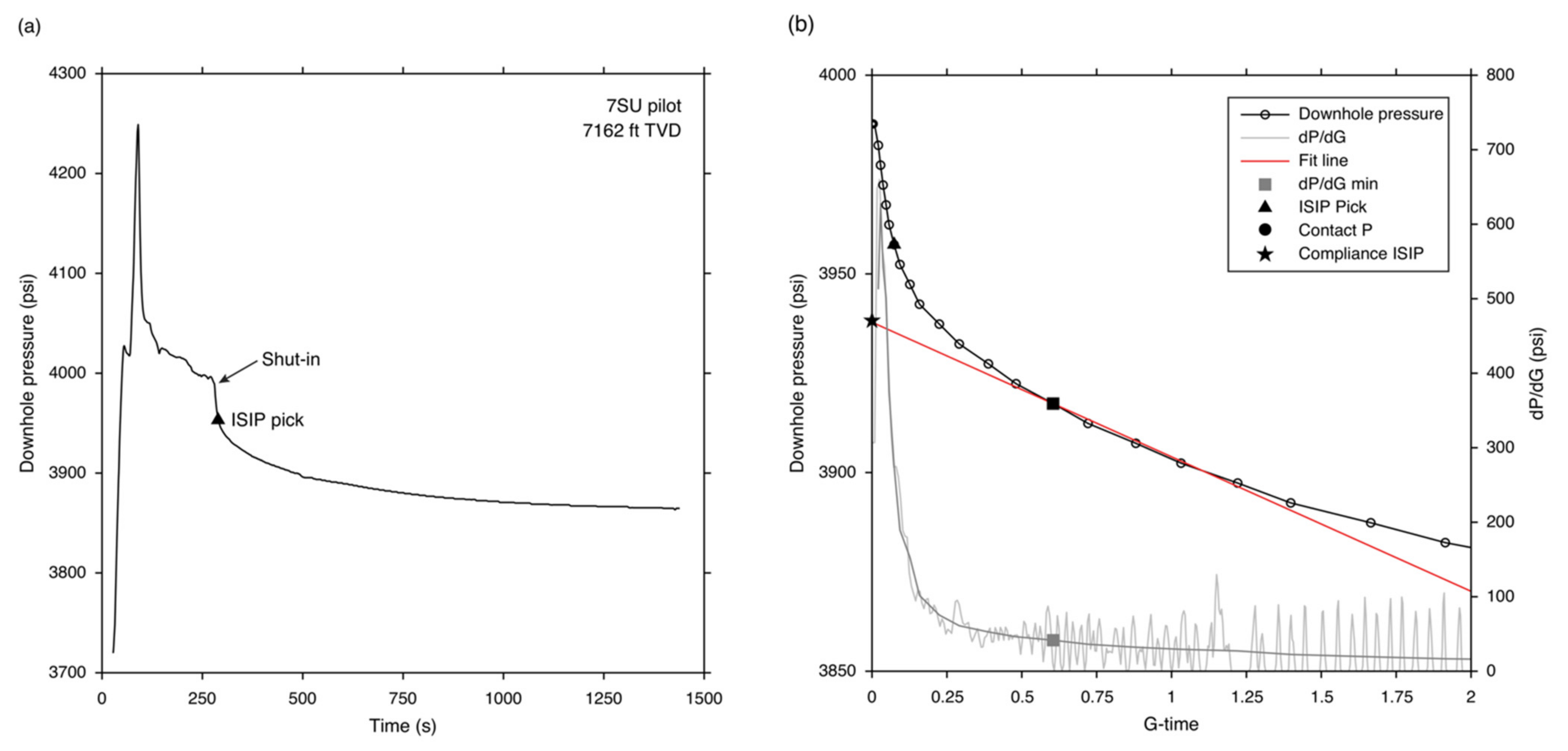
We estimated the value of Shmin from DFIT tests by both visually picking the value of the instantaneous shut-in pressure (ISIP) and by the compliance method [15]. Figure A1 shows an example of this analysis for a DFIT in the 7SU pilot well at 7162 ft TVD.
Figure A1.
DFIT test at 7162 ft TVD in the 7SU pilot well. (a) Downhole pressure record before and after shut in. Triangle symbol represents the value of the instantaneous shut in pressure (ISIP) picked visually. (b) Downhole pressure after shut in plotted as a function of G-time. Star symbol represents the ISIP determined from the compliance method [15].

Appendix A.2. Stratigraphic Alignment of Horizontal Wells
Figure A2.
Stratigraphic shift for the Upper Wolfcamp (-SU) wells. (a) Wells in cross section, not shifted by stratigraphic depth with respect to the 7SU pilot well. (b) Gamma ray logs from horizontal wells 3SU–8SU and the 7SU pilot well. Solid lines indicate the location of formation tops correlated with the 7SU pilot well. Dashed lines indicate the interpreted depth of formation tops based on the stratigraphic difference with respect to the 7SU pilot well.

Figure A3.
Stratigraphic shift for the Upper Wolfcamp (-SU) wells. (a) Wells in cross section, not shifted by stratigraphic depth with respect to the 7SU pilot well. (b) Gamma ray logs from horizontal wells 3SU–8SU and the 7SU pilot well. Solid lines indicate the location of formation tops correlated with the 7SU pilot well. Dashed lines indicate the interpreted depth of formation tops based on the stratigraphic difference with respect to the 7SU pilot well.

Appendix A.3. Instantaneous Shut-In Pressures (ISIPs)
ISIP values from hydraulic fracturing stages provide some indication of variations in Shmin. ISIP values cannot directly estimate Shmin because they incorporate near wellbore effects that add resistance to the measurement of formation stress. We estimated ISIPs for each of the 434 stages in order to provide secondary data in support of the DFITs and to explore variations in stress along the length of each horizontal well (e.g., Ma and Zoback, 2020).
Figure A4.
(a) Well trajectories in cross section shifted according to stratigraphic depth with respect to the pilot well (Figure A2 and Figure A3). (b) Ternary composition as a function of depth in the pilot well derived from Fourier transform infrared spectroscopy. (c) Clay + total organic carbon (TOC) as a function of depth. Regions exceeding 25 wt% are highlighted in black. (d) Stress, mudweight, and pore pressure as a function of depth. Measurements of Shmin are from DFITs in the pilot well and the toes of several horizontal wells (Figure A1). Stress measurements in both the Upper and Middle Wolfcamp are shifted according to stratigraphic depth with respect to the pilot well.

For each horizontal well, we averaged ISIP values over 10 ft intervals in TVD, with the bars on each point in Figure A4 representing the maximum and minimum values in the specific TVD interval. After shifting the depth of the averaged values according to the pilot well stratigraphy, the ISIP values are generally consistent with DFIT values from the horizontal wells and also indicate relatively high values of Shmin in clay + TOC-rich strata. The consistent relationship between stress variations and clay + TOC in the pilot well and in the stratigraphically shifted data demonstrates that in this part of the Wolfcamp rock composition is a reliable indicator of whether a given strata is at or above frictional equilibrium.
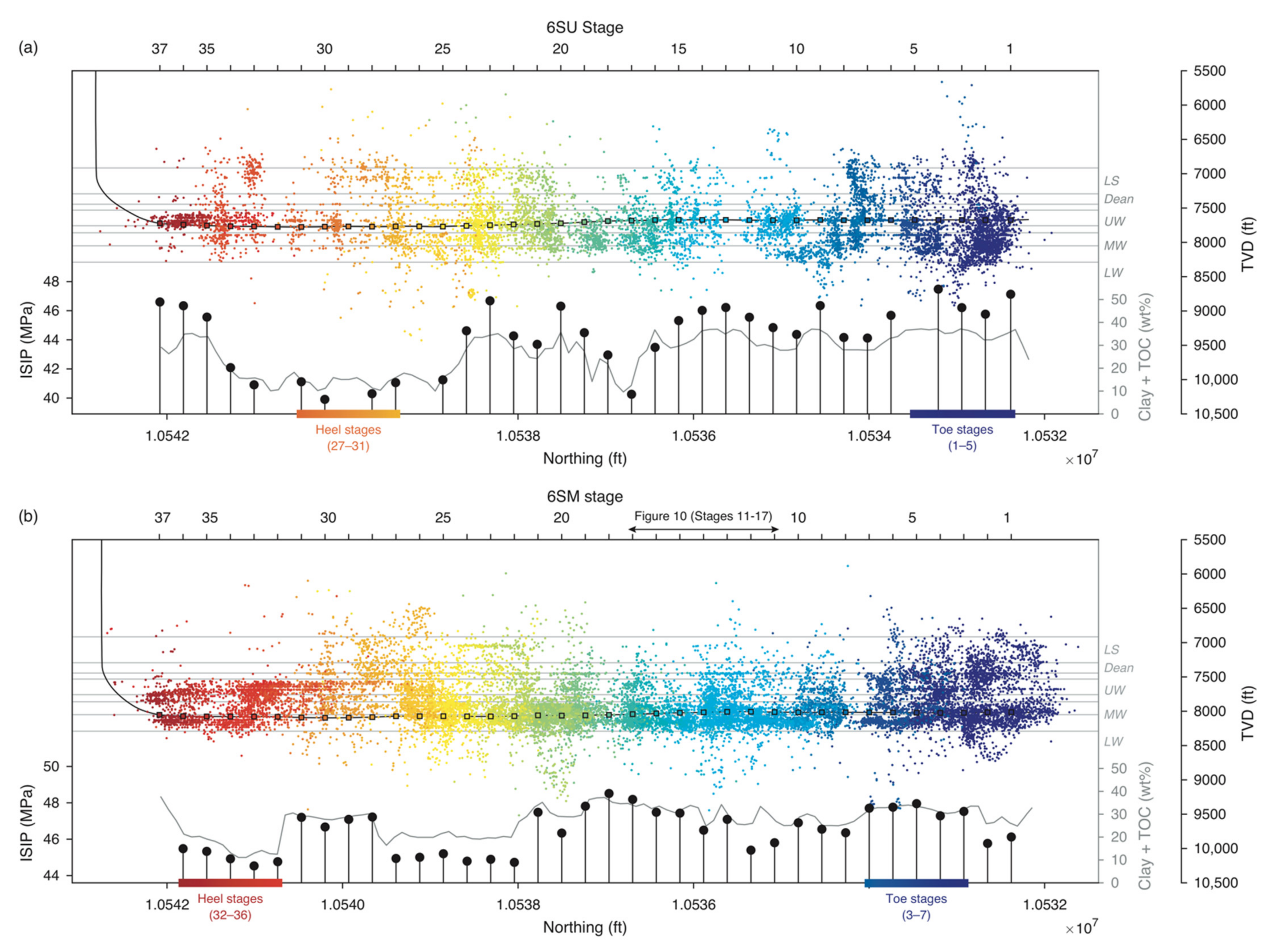
Figure A5a shows the variations in ISIP values and clay + TOC across well 6SU. The clay + TOC values are interpolated from the compositional log in the pilot well (Figure 4c) based on the stratigraphically shifted depths of the stages in well 6SU. The ISIP values appear positively correlated with clay + TOC. In this case, the stage-to-stage variations (~2–3 MPa) are ~2–4 times smaller than the variations in DFITs between the major strata (~8–10 MPa). Figure A5b shows the variations in ISIP values and clay + TOC across well 6SM. As in well 6SU, the ISIP values also appear positively correlated with clay + TOC.
Figure A5.
Horizontal profiles showing microseismicity, composition, and fracture stage instantaneous shut-in pressures (ISIPs) for wells (a) 6SU and (b) 6SM. Microseismic events colored by stage, ISIPs (black points), and clay + TOC (grey line) plotted over the well trajectory (black line). Colored squares represent stage locations. Clay + TOC values are interpolated from the compositional log in the 7SU pilot well.

Appendix A.4. Estimating the Value of SHmax
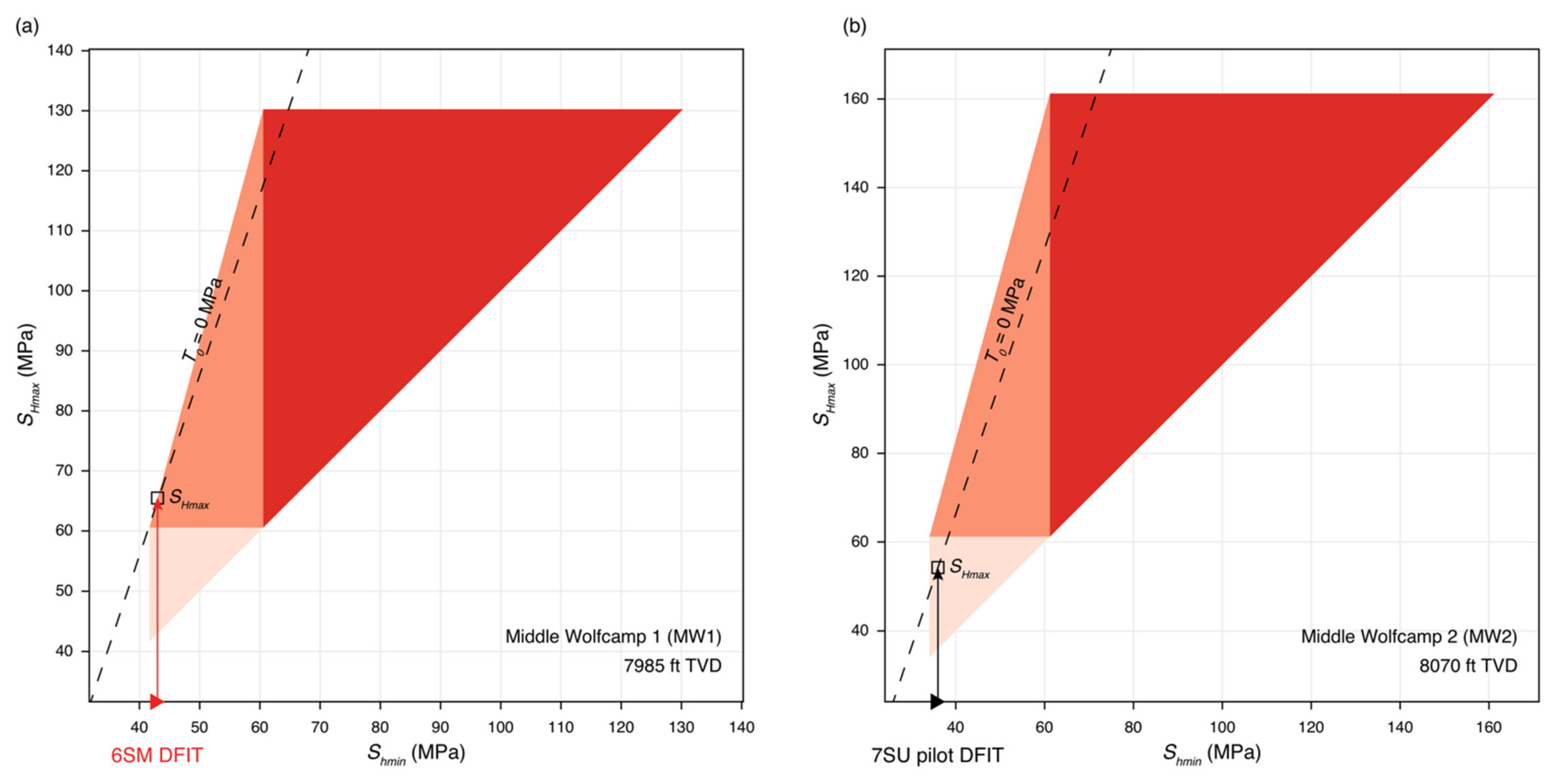
We estimated the value of SHmax for two points in the MW based on observations of no drilling induced tensile fractures in the image log for well 6SM. In each case, our estimated value of SHmax was the intersection of the Shmin line with tensile failure criterion (T0 = 0). The SHmax estimates are used in the fracture analysis (Figure 8, Figure 11 and Figure 12).
Figure A6.
Stress polygon diagrams corresponding to DFIT measurements at (a) the toe of horizontal well 6SM at 7985 ft TVD (b) in vertical pilot well 7SU at 8070 ft TVD.
Figure A6.
Stress polygon diagrams corresponding to DFIT measurements at (a) the toe of horizontal well 6SM at 7985 ft TVD (b) in vertical pilot well 7SU at 8070 ft TVD.

References
- Sone, H.; Zoback, M.D. Mechanical properties of shale-gas reservoir rocks—Part 2: Ductile creep, brittle strength, and their relation to the elastic modulus. Geophysics 2013, 78, D393–D402. [Google Scholar] [CrossRef]
- Sone, H.; Zoback, M.D. Time-dependent deformation of shale gas reservoir rocks and its long-term effect on the in situ state of stress. Int. J. Rock Mech. Min. Sci. 2014, 69, 120–132. [Google Scholar] [CrossRef]
- Sone, H.; Zoback, M.D. Viscous relaxation model for predicting least principal stress magnitudes in sedimentary rocks. J. Pet. Sci. Eng. 2014, 124, 416–431. [Google Scholar] [CrossRef]
- Xu, S.; Rassouli, F.S.; Zoback, M.D. Utilizing a viscoplastic stress relaxation model to study vertical hydraulic fracture propagation in the Permian Basin. In Proceedings of the SPE/AAPG/SEG Unconventional Resources Technology Conference, Austin, TX, USA, 24–26 July 2017; pp. 1–5. [Google Scholar]
- Singh, A. Stress Layering, Fault Slip and Hydraulic Fracture Propagation: Integrating Field Studies, Laboratory Experiments, and Numerical Simulations. 2021. Available online: https://www.proquest.com/openview/1f32cf4c7726712305f1d99eca2da577/1.pdf?pq-origsite=gscholar&cbl=18750&diss=y (accessed on 23 November 2021).
- Singh, A.; Zoback, M.; McClure, M. Optimization of multi-stage hydraulic fracturing in unconventional reservoirs in the context of stress variations with depth. In Proceedings of the SPE Annual Technical Conference and Exhibition, Denver, CO, USA, 5–7 October 2020. [Google Scholar]
- Ma, X.; Zoback, M.D. Predicting lithology-controlled stress variations in the Woodford shale from well log data via viscoplastic relaxation. SPE J. 2020, 25, 2534–2546. [Google Scholar] [CrossRef]
- McCormack, K.; Zoback, M.; Kuang, W. A case study of vertical hydraulic fracture growth, stress variations with depth and shear stimulation in the Niobrara shale and Codell sand, DJ Basin, Colorado. Interpretation 2021, 9, 1N-T1196. [Google Scholar] [CrossRef]
- Ciezobka, J.; Courtier, J.; Wicker, J. Hydraulic fracturing test site (HFTS)—Project overview and summary of results. In Proceedings of the SPE/AAPG/SEG Unconventional Resources Technology Conference, Houston, TX, USA, 23–25 July 2018; pp. 1–9. [Google Scholar]
- Snee, J.E.L.; Zoback, M.D. State of stress in the Permian Basin, Texas and New Mexico: Implications for induced seismicity. Lead. Edge 2018, 37, 127–134. [Google Scholar] [CrossRef] [Green Version]
- Lund Snee, J.-E.; Zoback, M. State of stress in areas of active unconventional oil and gas development in North America. Am. Assoc. Pet. Geol. Bull. 2021. In press. [Google Scholar] [CrossRef]
- Simpson, R.W. Quantifying Anderson’s fault types. J. Geophys. Res. 1997, 102, 17909–17919. [Google Scholar] [CrossRef]
- U.S. Energy Information Administration. Permian Basin: Wolfcamp Shale Play Geology Review; U.S. Energy Information Administration: Washington, DC, USA, 2018.
- Maity, D. Microseismicity analysis for HFTs pad and correlation with completion parameters. In Proceedings of the SPE/AAPG/SEG Unconventional Resources Technology Conference, Houston, TX, USA, 23–25 July 2018; pp. 1–12. [Google Scholar] [CrossRef]
- McClure, M.; Bammidi, V.; Cipolla, C.; Cramer, D.; Martin, L.; Savitski, A.A.; Sobernheim, D.; Voller, K. A collaborative study on DFIT interpretation: Integrating modeling, field data, and analytical techniques. In Proceedings of the SPE/AAPG/SEG Unconventional Resources Technology Conference, Denver, CO, USA, 22–24 July 2019; pp. 1–39. [Google Scholar] [CrossRef]
- Zoback, M.D.; Kohli, A.H. Unconventional Reservoir Geomechanics; Cambridge University Press: Cambridge, UK, 2019; ISBN 9781107087071. [Google Scholar]
- Kohli, A.H.; Zoback, M.D. Frictional properties of shale reservoir rocks. J. Geophys. Res. Solid Earth 2013, 118, 5109–5125. [Google Scholar] [CrossRef]
- Gale, J.F.W.; Elliott, S.J.; Laubach, S.E. Hydraulic fractures in core from stimulated reservoirs: Core fracture description of HFTs slant core, Midland Basin, West Texas. In Proceedings of the SPE/AAPG/SEG Unconventional Resources Technology Conference, Houston, TX, USA, 23–25 July 2018. [Google Scholar]
- Elliott, S.J.; Gale, J.F.W. Analysis and distribution of proppant recovered from fracture faces in the HFTS slant core drilled through a stimulated reservoir. In Proceedings of the SPE/AAPG/SEG Unconventional Resources Technology Conference, Houston, TX, USA, 23–25 July 2018. [Google Scholar]
- Kuang, W.; Zoback, M.; Zhang, J. Estimating geomechanical parameters from microseismic plane focal mechanisms recorded during multistage hydraulic fracturing. Geophysics 2017, 82, KS1–KS11. [Google Scholar] [CrossRef]
Figure 1.
(a) Regional stress map showing the location of the Hydraulic Fracture Test Site-1 (HTFS-1) in an area of strike-slip/normal faulting (adapted from Lund Snee and Zoback, 2018, 2020). The direction of the maximum horizontal compressive stress, SHmax, (black lines) is approximately E-W. (b) A vertical pilot well (7SU pilot) and a ‘wine rack’ pattern of horizontal wells were drilled N to S into the Upper (-SU) and Middle Wolfcamp (-SM) shale units. After hydraulic fracturing, a deviated well (6TW) was drilled through the stimulated volume.2.2. Well Logs, Core, and Microseismic Data.

Figure 2.
(a) Cross section of well trajectories in the Upper and Middle Wolfcamp. Slant well 6TW was cored in two locations (cores 1–4 and 5–6), indicated by the grey boxes on the well trajectory. Grey lines indicate formation tops designed in the 7SU pilot well. LS: Lower Sprayberry, UW: Upper Wolfcamp, MW: Middle Wolfcamp, LW: Lower Wolfcamp. (b) Stress profile incorporating measurements of drilling mudweight and diagnostic formation integrity tests (DFITs) in both vertical and horizontal wells. Grey area shows Shmin predicted by frictional equilibrium for friction coefficients, μ = 0.6–0.8. (c) Mohr circles representing the variation in stress state in the UW2 unit at 7769–7703 ft based on DFIT measurements from horizontal wells 4SU, 6SU, and 8SU. (d) Mohr circle representing the stress state in the UW3 unit at 7790 ft based on DFIT measurements in the 7SU pilot well.

Figure 3.
(a) N-S cross section of microseismic events generated by hydraulically fracturing horizontal wells in the Upper and Middle Wolfcamp. Events are colored by the stage where they were generated. Each well has between 37–49 stages. (b) Histogram of event depths from all stages.
Figure 3.
(a) N-S cross section of microseismic events generated by hydraulically fracturing horizontal wells in the Upper and Middle Wolfcamp. Events are colored by the stage where they were generated. Each well has between 37–49 stages. (b) Histogram of event depths from all stages.

Figure 4.
(a) Well trajectories in cross section shifted according to stratigraphic depth with respect to the pilot well (Figure A1). (b) Clay + total organic carbon (TOC) as a function of depth. Regions with clay + TOC exceeding 25 wt% are highlighted in black. (c) Stress, mudweight, and pore pressure as a function of depth. Measurements of Shmin include DFITs from the vertical pilot well and horizontal wells. Stress measurements in both the Upper and Middle Wolfcamp are shifted according to stratigraphic depth with respect to the pilot well. The black line is the interpreted stress profile based on stratigraphically shifted stress measurements and is dashed in the regions with no data.

Figure 5.
Relationship between stress, composition, and seismicity in well 6SU. (a) Interpreted stress profile including DFITs from vertical wells (black triangles), DFITs from horizontal wells (colored triangles), and instantaneous shut-in pressure (ISIP) for 6SU stages 1–5 (blue points) and 27–31 (red points). ISIP values are expected to be ~3–5 MPa higher than DFITs. (b) Clay + TOC in the 7SU pilot well. (c) Distribution of microseismic events colored by stage from the five toe stages (blue) and five heel stages (red to orange). (d) Histogram of microseismic event depths from the five toe stages (blue) and five heel stages (red to orange).

Figure 6.
Relationship between stress, composition, and seismicity in well 6SM. (a) Interpreted stress profile including DFITs from vertical wells (black triangles), DFITs from horizontal wells (colored triangles), and instantaneous shut-in pressure (ISIP) for 6SU stages 3–7 (blue points) and 32–36 (red points). ISIP values are expected to be ~3–5 MPa higher than DFITs. (b) Clay + TOC in the 7SU pilot well. (c) Distribution of microseismic events colored by stage from the five toe stages (blue) and five heel stages (red to orange). (d) Histogram of microseismic event depths from the five toe stages (blue) and five heel stages (red to orange).

Figure 7.
Fracture data from image logs and recovered core. (a) Upper Wolfcamp fractures. Natural fractures identified in well 6SU. Number of fractures, N = 503. Natural fractures (N = 148) and hydraulic fractures (N = 134) identified in well 6TW cores 1–4. (b) Middle Wolfcamp fractures. Natural fractures identified in well 6SM (N = 1012). Natural fractures (N = 23) and hydraulic fractures (N = 33) identified in well 6TW cores 5–6.

Figure 8.
(a) Interpreted stress profile based on stratigraphically shifted stress measurements. (b–e) Mohr circle diagrams for stress layers in the Upper and Middle Wolfcamp. In each diagram, the fractures that are plotted represent the sum of observations from image logs (wells 6SU, 6SM, and 7SU) and from core samples from slant core well 6TW. Red points represent the population of fractures that are activated if pore pressure is raised to the value of Shmin. PPcrit is the pressure needed to active faults given a coefficient friction of 0.7 and PPmax is the maximum possible pressure, i.e., Shmin.

Figure 9.
Relationships between hydraulic stimulation and microseismicity. (a) Pressure–rate–time plots for well 6SM Stages 1, 5, and 34. Black arrows indicate origin point for injection. ISIP values are indicated by black triangles. (b) Microearthquake distance-plots for well 6SM Stages 1, 5, and 34. Points are sized by magnitude and colored by time after injection. The dashed line indicates an average hydraulic fracture propagation velocity, ~2000 ft/hr.

Figure 10.
(a) Interpreted stress profile based on stratigraphically shifted stress measurements. ISIP values for well 6SM stages 1, 5, and 34 are plotted as small red triangles. (b–d) Gun barrel views of microseismicity from stages 1, 5, and 34. Events are colored by time after injection (Figure 10). White stars indicate the location of each stage.

Figure 11.
Earthquake focal mechanisms for well 6SM. (a) All microseismic events colored by stage (colored points). Events with moment tensor solutions in stages 11–17 sized by magnitude (red points). (b) Histogram of fractures observed in image logs in pilot well 7SU. (c) Stereonet of active fractures observed in image logs in horizontal wells 6SU and 6SM. Arrows indicate the direction of the maximum compressive stress, SHmax. (d) Stereonet of inactive fractures. (e) Stereonet of primary nodal planes from the focal mechanism (FM) inversion.

Figure 12.
Relationships between stimulation, spatiotemporal distribution of seismicity, and microseismic source mechanisms for well 6SM stage 14. (a) Pressure–rate–time plot showing the start of injection (black arrow) and the value of the instantaneous shut-in pressure (ISIP). (b) Distance–time plot showing earthquakes colored by time after injection and sized by relative magnitude. Five specific earthquakes with moment tensor solutions are highlighted. (c) Stress profile and gun barrel view of microearthquake distribution. Events are colored by time after injection and sized by relative magnitude. (d) Mohr diagram representing stress state for well 6SM. The five events are plotted as well as the interpreted fault plane from Stg 1. Red points represent potentially active faults from the fracture dataset. Grey points represent faults unable to be activated for this stress state. (e) Stereonet of the interpreted fault plane from Stage 1 and the five highlighted faults colored by time after injection. The rake of the slip vector is listed for each event. Arrows indicate the direction of the maximum compressive stress, SHmax.

Publisher’s Note: MDPI stays neutral with regard to jurisdictional claims in published maps and institutional affiliations. |
© 2021 by the authors. Licensee MDPI, Basel, Switzerland. This article is an open access article distributed under the terms and conditions of the Creative Commons Attribution (CC BY) license (https://creativecommons.org/licenses/by/4.0/).
Share and Cite
MDPI and ACS Style
Kohli, A.; Zoback, M. Stratigraphically Controlled Stress Variations at the Hydraulic Fracture Test Site-1 in the Midland Basin, TX. Energies 2021, 14, 8328. https://doi.org/10.3390/en14248328
AMA Style
Kohli A, Zoback M. Stratigraphically Controlled Stress Variations at the Hydraulic Fracture Test Site-1 in the Midland Basin, TX. Energies. 2021; 14(24):8328. https://doi.org/10.3390/en14248328
Chicago/Turabian StyleKohli, Arjun, and Mark Zoback. 2021. "Stratigraphically Controlled Stress Variations at the Hydraulic Fracture Test Site-1 in the Midland Basin, TX" Energies 14, no. 24: 8328. https://doi.org/10.3390/en14248328
Note that from the first issue of 2016, this journal uses article numbers instead of page numbers. See further details here.